Wavelet-Based Entropy Measures to Characterize Two-Dimensional Fractional Brownian Fields

Abstract

The aim of this work was to extend the results of Perez et al. (Physica A (2006), 365 (2), 282–288) to the two-dimensional (2D) fractional Brownian field. In particular, we defined Shannon entropy using the wavelet spectrum from which the Hurst exponent is estimated by the regression of the logarithm of the square coefficients over the levels of resolutions. Using the same methodology. we also defined two other entropies in 2D: Tsallis and the Rényi entropies. A simulation study was performed for showing the ability of the method to characterize 2D (in this case, $\alpha =2$) self-similar processes.

1. Introduction

The concept of entropy was first introduced by [1] in thermodynamics as a measure of the amount of energy in a system. Posteriorly, Boltzmann [2] was the first who gave a probabilistic interpretation, setting the foundations of statistical physics. Shannon [3] proposed the entropy concept on the subject of information theory as the average rate at which information is produced by a stochastic data source. According to information theory, entropy is a measure of uncertainty and unpredictability associated with a random variable (discrete or continuous), and Shannon entropy quantifies the expected value of information generated from a random variable. The definition of entropy has been widely used in many applications, such as neural systems [4], image segmentation through thresholding [5,6], climatology, and hydrology [7,8,9,10]. Nicholson et al. [11] introduced spatial entropy to study earthquake distributions. A temporal definition of entropy was used by [12,13,14,15] to study seismicity in different parts of the world.

For a process characterized by a certain number N of states or classes of events, Shannon entropy [3] is defined as

$$S=-\sum _{i=1}^N{p}_{i}log(p_i),$$

(1)

where $p_i$ is the probability of event occurrence in each i-th class. The choice of the base of the logarithm is arbitrary: for practical convenience, we used base two throughout this paper ($log\equiv {log}_2$). For $p_i=0$, $p_i{log}_2{p}_i=0$. Shannon entropy is maximal when all outcomes are equally likely, that is, $S={log}_2(N)$.

A generalization of Shannon entropy is Rényi entropy proposed by [16] as

$$S_{\alpha }=\frac{1}{1-\alpha }{log}_2\left(\sum _{i=1}^N{p}_i^{\alpha }\right),$$

(2)

where $\alpha$, $\alpha >1$, is a parameter. Shannon entropy is obtained from $S_{\alpha }$ as $\alpha \to 1$ (see, e.g., [17]), and Rényi entropy is non-negative in discrete Case (2). Finally, for any ${\alpha }_1<{\alpha }_2$, we have $S_{{\alpha }_1}\ge S_{{\alpha }_2}$ (and $S_{{\alpha }_1}=S_{{\alpha }_2}$ if and only if the system is uniformly distributed).

Another generalization of Shannon entropy is Tsallis entropy, proposed by [18] as

$$T_{\alpha }=\frac{1}{\alpha -1}\left(1-\sum _{i=1}^N{p}_i^{\alpha }\right).$$

(3)

Tsallis entropy satisfies the following properties: (i) $T_{\alpha }\ge 0$ with $(\alpha -1)T_{\alpha }\le 1$; (ii) $T_{\alpha }\to S$ as $\alpha \to 1$; (iii) pseudoadditivity between two independent systems A and B: $T_{\alpha }(A,B)=T_{\alpha }(A)+T_{\alpha }(B)+(1-\alpha )T_{\alpha }(A)T_{\alpha }(B)$ (additivity is accomplished if $\alpha =1$); and (iv) it is a non-decreasing function of the Rényi entropy because [19]

$$S_{\alpha }=\frac{1}{1-\alpha }{log}_2[1+(1-\alpha )T_{\alpha }].$$

However, probability density is not the only type of distribution that can give information, and the definition of entropy can be extended to other types of distributions, such as energy distribution based on wavelet coefficients [20]. A definition of Shannon wavelet entropy based on the energy distribution of wavelet coefficients was proposed by [21,22,23,24,25,26,27]. In particular, Sello [21] defined temporal wavelet entropy using continuous wavelets, and [20] introduced multiresolution wavelet entropy by summing the energy for all discrete times, and discretizing scale j. Nicolis and Mateu [28] used the anisotropic Morlet wavelet to define Shannon entropy in two-dimensional point processes. A discrete version of Shannon wavelet entropy was proposed by [25,26,27,29,30,31,32] to characterize self-similar processes with Gaussian and stationary increments. Recently, a similar approach based on wavelet probability densities was proposed by [33] using the Fisher–Shannon method [15].

However, the latter authors used a definition of wavelet entropy for characterizing self-similar processes in the time domain, but an extension to the two-dimensional case has not been proposed so far. In this work, we extend the definition of wavelet Shannon entropy proposed by [25,26,27] to provide a characterization of an isotropic n-dimensional fractional Brownian field. The same methodology is also used for defining wavelet-based Rényi and Tsallis entropies. A simulation study is provided to prove and check the results.

The article is organized as follows: Section 2 provides some basic concepts of fractional Brownian motion and its extensions. Section 3 gives some definitions of 2D wavelet transforms. Directional wavelets and anisotropic wavelet entropy are introduced in Section 4. A simulation study is reported in Section 5. The paper ends with some conclusions in Section 6.

2. Fractional Brownian Motion and Extensions

Fractional Brownian motion (fBm) denoted by $\{B_H(t),t\in \mathbb{R}\}$, is a Gaussian, zero-mean, nonstationary stochastic process originally proposed by [34]. This process is called self-similar since, for all $a>0$, it satisfies

$$B_H(at)\stackrel{d}{=}{a}^H{B}_H(t),$$

where H is the self-similarity or Hurst exponent parameter, and “$\stackrel{d}{=}$” denotes equality in distribution. The fBm process is characterized by the following covariance function:

$$R_{B_H}(t,s)=E\left\{B_H(t)B_H(s)\right\}=\frac{{\sigma }_H^2}{2}\left[{\left|t\right|}^{2H}+{\left|s\right|}^{2H}-{|t-s|}^{2H}\right],$$

(4)

where

$${\sigma }_H^2=\Gamma (1-2H)\frac{cos(\pi H)}{\pi H},0<H<1.$$

As can be seen from Function (4), the fBm is a nonstationary process, but with stationary increments. These definitions can be extended to any dimension. The case of fBm generalization from one to higher dimensions is not unique. A simple generalization to a 2D surface is the fractional Brownian field (fBf). The fBf is a Gaussian, zero-mean, random field $B_H(\mathbf{u})$, where $\mathbf{u}$ denotes the position in a selected domain, usually $[0,1]\times [0,1]$. Its covariance function is given by

$$R_{B_H}(\mathbf{u},\mathbf{v})=E\left[B_H(\mathbf{u})B_H(\mathbf{v})\right]=\frac{{\sigma }_H^2}{2}\left({∥\mathbf{u}∥}^{2H}+{∥\mathbf{v}∥}^{2H}+{∥\mathbf{u}-\mathbf{v}∥}^{2H}\right),$$

(5)

where $0<H<1$, the variance ${\sigma }_H^2$ is

$${\sigma }_H^2=\frac{2^{-(1+2H)}\Gamma (1-H)}{\pi H\Gamma (1+H)},$$

(6)

and $∥·∥$ is the usual Euclidean norm in ${\mathbb{R}}^2$ (see [35,36,37]). The increments of an fBf represent stationary, zero-mean, Gaussian random fields because the variance of such increments only depends on distance $∥\mathbf{h}∥$ so that

$$E{\left[B_H(\mathbf{u}+\mathbf{h})-B_H(\mathbf{u})\right]}^2={\sigma }_H^2{\parallel \mathbf{h}\parallel }^{2H},$$

where ${\sigma }_H^2$ is given in Equation (6).

The extension to the d-dimensional case is straightforward [38]. For a d-dimensional fractional Brownian motion, the covariance function is given by Equation (5) with $\mathbf{u},\mathbf{v}$ in ${\mathbb{R}}^d$, and

$${\sigma }_H^2=\frac{2^{-1-d-2H}\Gamma (1-H)}{{\pi }^{\frac{d}{2}}H\Gamma (\frac{d}{2}+H)}.$$

(7)

Although many generalizations have been proposed to include anisotropy in Gaussian random fields [37,39], in the following section, we only consider the isotropic version of the fBf.

3. Two-Dimensional Wavelet Transforms

In one or higher dimensions, wavelets provide an appropriate tool for analyzing self-similar signals or objects. In the two-dimensional domain, wavelet transforms can be constructed through translations and the dyadic scaling of a product of univariate wavelets and scaling functions. Using the same setting as that provided in [35], the following so-called separable 2D wavelets can be defined as

$$\begin{array}{cc}\hfill \varphi (u_x,u_y)& =\varphi (u_x)·\varphi (u_y),\hfill \\ \hfill {\psi }^h(u_x,u_y)& =\varphi (u_x)·\psi (u_y),\hfill \\ \hfill {\psi }^v(u_x,u_y)& =\psi (u_x)·\varphi (u_y),\hfill \\ \hfill {\psi }^d(u_x,u_y)& =\psi (u_x)·\psi (u_y),\hfill \end{array}$$

where $\varphi$ and $\psi$ are scaling and wavelet functions, and symbols $h,v,d$ stand for the horizontal (h), vertical (v), and diagonal (d) directions, respectively. So, any function $g\in L^2({\mathbb{R}}^2)$ has the following representation:

$$g(\mathbf{u})=\sum _{\mathbf{k}=(k_1,k_2)}{c}_{j_0,\mathbf{k}}{\varphi }_{j_0,\mathbf{k}}(\mathbf{u})+\sum _{j\ge j_0}\sum _{\mathbf{k}=(k_1,k_2)}\sum _{i=h,v,d}{d}_{j,\mathbf{k}}^i{\psi }_{j,\mathbf{k}}^i(\mathbf{u}),$$

(8)

with $\mathbf{u}=(u_x,u_y)\in {\mathbb{R}}^2$, $(k_1,k_2)\in {\mathbb{Z}}^2$, ${\varphi }_{j,\mathbf{k}}(\mathbf{u})$ and ${\psi }_{j,\mathbf{k}}(\mathbf{u})$ being the translations and dilations of the scaling function and of the mother wavelet, defined by

$$\begin{array}{ccc}\hfill {\varphi }_{j,\mathbf{k}}(\mathbf{u})& =& 2^{2j}\varphi (2^j{u}_x-k_1,2^j{u}_y-k_2),\hfill \\ \hfill {\psi }_{j,\mathbf{k}}^i(\mathbf{u})& =& 2^{2j}{\psi }^i(2^j{u}_x-k_1,2^j{u}_y-k_2),\hfill \end{array}$$

for $i=h,v,d$ [40]. The scaling and detail coefficients in Equation (8), respectively, are given by

$$\begin{array}{cc}\hfill c_{j,\mathbf{k}}& =\langle g,{\varphi }_{j,\mathbf{k}}\rangle =2^{2j}{\int }_{{\mathrm{I}\mathrm{R}}^2}g(\mathbf{t})\varphi (2^j\mathbf{t}-\mathbf{k})d\mathbf{t},\hfill \\ \hfill d_{j,\mathbf{k}}^i& =\langle g,{\psi }_{j,\mathbf{k}}\rangle =2^{2j}{\int }_{{\mathrm{I}\mathrm{R}}^2}g(\mathbf{t}){\psi }^i(2^j\mathbf{t}-\mathbf{k})d\mathbf{t},\hfill \end{array}$$

for $i=h,v,d$. With this notation, $j_0$ denotes the coarsest scale and therefore the lowest resolution in the representation. A larger j corresponds to a finer scale, and therefore corresponds to a higher resolution. If $M\times M$ is the size of the matrix representing a 2D object (for example, an image), the number of coefficients for each level of resolution and direction i is $2^{j}M\times 2^{j}M$ with $j=-N,\dots ,-1$ and $N={log}_2(M)$, where M must be taken a priori to be an integer power of 2, i.e., $M=2^N$. For further details on wavelet theory, see [40,41]. Wavelet transform can be also extended to the $n-$dimensional case (see, for example, [42] for a 3D case).

4. Shannon Wavelet Entropy for 2D FBF

In this section, in order to address Shannon wavelet entropy for a 2D fBf, we deal with a random signal (with some second-order properties) for wavelet energy to be written in terms of expectations. Following the notation of [26] for the one-dimensional case, 2D wavelet energy at resolution j can be written as

$$E^i(j)=\sum _{\mathbf{k}=(k_1,k_2)}\mathbb{E}[|d_{j,\mathbf{k}}^i{|}^2],$$

and 2D relative wavelet energy (RWE) is given by

$$p^i(l)=\frac{E^i(l)}{{\sum }_{l=-N}^{-1}{E}^i(l)}=\frac{{\sum }_{\mathbf{k}=(k_1,k_2)}\mathbb{E}[|d_{l,\mathbf{k}}^i{|}^2]}{{\sum }_{l=-N}^{-1}{\sum }_{\mathbf{k}=(k_1,k_2)}\mathbb{E}[|d_{l,\mathbf{k}}^i{|}^2]},$$

(9)

for varying index l, $l=-N\dots -1$, being N is the maximal resolution level.

Consequently, 2D normalized Shannon, Rényi, and Tsallis wavelet entropies (NSWE, NRWE, and NTWE, respectively) can be defined as

$$\begin{array}{ccc}\hfill S^i& =& -\frac{1}{{log}_{2}N}\sum _{l=-N}^{-1}{p}^i(l){log}_2(p^i(l)),\hfill \end{array}$$

(10)

$$\begin{array}{ccc}\hfill S_{\alpha }^i& =& \frac{{log}_2\left({\sum }_{l=-N}^{-1}{[p^i(l)]}^{\alpha }\right)}{(1-\alpha ){log}_{2}N},\hfill \end{array}$$

(11)

$$\begin{array}{ccc}\hfill T_{\alpha }^i& =& \frac{1-{\sum }_{l=-N}^{-1}{[p^i(l)]}^{\alpha }}{(\alpha -1){log}_{2}N},\hfill \end{array}$$

(12)

respectively.

For an fBf process $B_H(\mathbf{x})$, the detail coefficients are random variables given by

$$d_{j,\mathbf{k}}^i=2^j{\int }_{{\mathrm{I}\mathrm{R}}^2}{B}_H(\mathbf{x}){\psi }^i(2^j\mathbf{x}-\mathbf{k})d\mathbf{x},$$

(13)

where $i=h,v$ or d. The detail coefficients have zero mean and variance (see [35,43]) given by

$$\mathbb{E}[|d_{j,\mathbf{k}}^i{|}^2]=2^{2j}{\int }_{{\mathrm{I}\mathrm{R}}^2}{\int }_{{\mathrm{I}\mathrm{R}}^2}{\psi }^i\left(2^j\mathbf{x}-\mathbf{k}\right){\psi }^i\left(2^j\mathbf{v}-\mathbf{k}\right)E\left[B_H(\mathbf{x})B_H(\mathbf{v})\right]d\mathbf{x}d\mathbf{v}.$$

(14)

From Equation (14), we can derive

$$\mathbb{E}[|d_{j,\mathbf{k}}^i{|}^2]=\frac{{\sigma }_H^2}{2}{V}_{{\psi }^i}{2}^{-(2H+2)j},$$

(15)

where

$$V_{{\psi }^i}=-{\int }_{{\mathrm{I}\mathrm{R}}^2}{\int }_{{\mathrm{I}\mathrm{R}}^2}{\psi }^i(\mathbf{p}+\mathbf{q})·{\psi }^i(\mathbf{q}){\left|\mathbf{p}\right|}^{2H}d\mathbf{p}d\mathbf{q}$$

(16)

with $\mathbf{p}=2j(\mathbf{x}-\mathbf{v})$ and $\mathbf{q}=2^j\mathbf{v}-\mathbf{k}$ (see [35], for the derivation of this result). (16) only depends on wavelets ${\psi }^i$ and exponent H, but not on scale j.

An application of the logarithm with base two to both sides of Expression (15) leads to the following equation:

$${log}_2\mathbb{E}[|d_{j,\mathbf{k}}^i{|}^2]=-(2H+2)j+C_i,$$

(17)

where

$$C_i={log}_2\left\{\frac{{\sigma }_H^2}{2}{V}_{{\psi }^i}(H)\right\}.$$

The Hurst coefficient of an fBf is estimated from the slope of the linear equation given in Equation (17). The empirical counterpart of Equation (17) is regression defined in pairs,

$$\left(j,{log}_2\overline{{\left|d_{j,\mathbf{k}}^i\right|}^2}\right),i=h,v,d,$$

(18)

where $\overline{{\left|d_{j,\mathbf{k}}^i\right|}^2}$ is an empirical counterpart of $E\left[{\left|d_{j,\mathbf{k}}^i\right|}^2\right]$ [35].

By replacing Equation (15) into 2D RWE (9), we obtain the relative wavelet energy at direction i for a 2D fractional Brownian field, that is,

$$p^i(l)=\frac{2^{-(2H+2)l}}{{\sum }_{l=-N}^{-1}{2}^{-(2H+2)l}},$$

(19)

for varying index l.

Since for isotropic processes, relative wavelet energy is independent of wavelet basis, $p^i(j)$ are equal for each direction $i=d,h,v$. However, it could be not true for general isotropic processes without the self-similarity condition. Next, we only considered the $d-$direction, and we denote by $p(j)$ its relative wavelet energy at each resolution j.

Proposition 1.

Let H be the Hurst exponent parameter and N the number of resolution levels, then:

$$\sum _{j=-N}^{-1}{2}^{-j(2+2H)}=2^{(2+2H)}\left(\frac{1-2^{-(2+2H)N}}{1-2^{-(2+2H)}}\right).$$

For proof of Proposition 1, see the Appendix A. For a 2D object of $M\times M$ size, and with a maximal resolution level already explicitly fixed to $N={log}_2(M)$, Equation (19) can be written using Proposition 1 as

$$p(j)=\left(\frac{1-2^{-(2+2H)}}{1-2^{-(2+2H)N}}\right)2^{-(2+2H)(j+1)}.$$

(20)

Similarly to the 1D case described in [27], by replacing Equation (19) in Equation (10), and considering $\gamma =1$ in Proposition 1, wavelet-based Shannon entropy for a grid-sampled fBf and fixing maximal resolution level N is given by

$$S(N,H)=\frac{1}{{log}_2(N)}(2+2H)\left[\frac{1}{2^{(2+2H)}-1}-\frac{N}{2^{(2+2H)N}-1}\right]-\frac{1}{{log}_2(N)}{log}_2\left[\frac{1-2^{-(2+2H)}}{1-2^{-(2+2H)N}}\right],$$

(21)

which only depends on H and N. Equation (21) can be easily generalized to m dimensions by using

$$E\left[{\left|d_{j,\mathbf{k}}^i\right|}^2\right]=2^{-(2H+m)}{\sigma }_H^2$$

in Equation (20), with

$${\sigma }_H^2=\Gamma (1-2H)\frac{cos(\pi H)}{\pi H},0<H<1.$$

Proposition 2.

Let H be the Hurst exponent parameter, N the number of resolution levels, and $\alpha >1$; then,

$$\sum _{j=-N}^{-1}{[p^i(j)]}^{\alpha }={\left(\frac{1-2^{-(2+2H)}}{1-2^{-(2+2H)N}}\right)}^{\alpha }\left(\frac{1-2^{-\alpha (2+2H)N}}{1-2^{-\alpha (2+2H)}}\right).$$

For a proof of Proposition 2, see the Appendix A. By replacing Equation (19) in Equations (11) and (12), and considering Proposition 2, wavelet-based Rényi and Tsallis entropies for a grid-sampled fBf and fixing maximal resolution level N are given by

$$\begin{array}{ccc}\hfill S_{\alpha }(N,H)& =& \frac{1}{(1-\alpha ){log}_{2}N}{log}_2\left\{{\left(\frac{1-2^{-(2+2H)}}{1-2^{-(2+2H)N}}\right)}^{\alpha }\left(\frac{1-2^{-\alpha (2+2H)N}}{1-2^{-\alpha (2+2H)}}\right)\right\},\hfill \end{array}$$

(22)

$$\begin{array}{ccc}\hfill T_{\alpha }(N,H)& =& \frac{1}{(\alpha -1){log}_{2}N}\left\{1-{\left(\frac{1-2^{-(2+2H)}}{1-2^{-(2+2H)N}}\right)}^{\alpha }\left(\frac{1-2^{-\alpha (2+2H)N}}{1-2^{-\alpha (2+2H)}}\right)\right\},\hfill \end{array}$$

(23)

respectively; both only depend on $\alpha$, H, and N.

5. Simulation Study

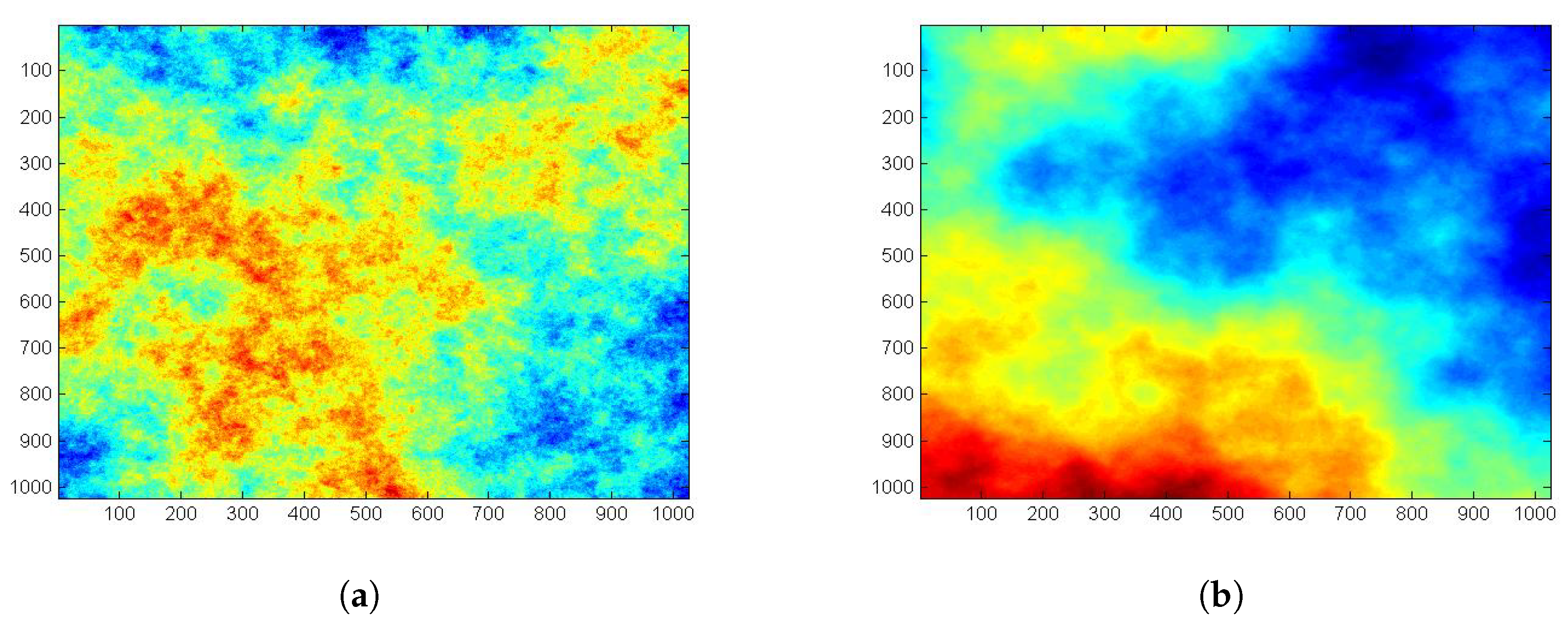
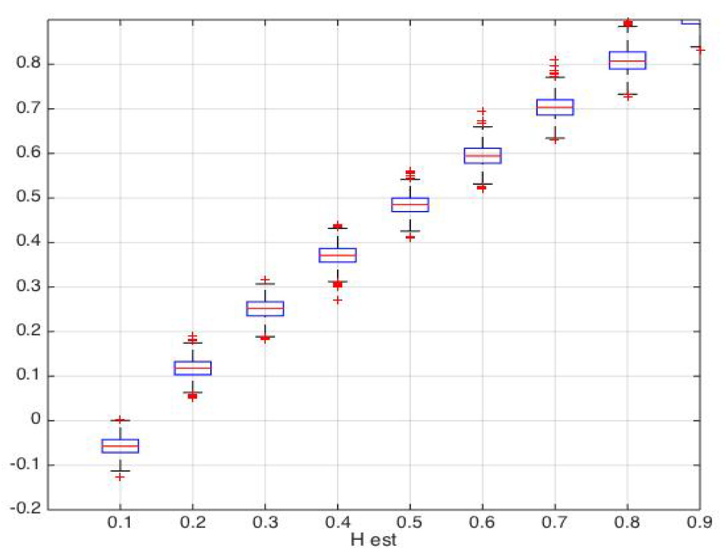
For illustrative purposes, we simulated $N=1000$ 2D fractional Brownian fields with $1024\times 1024$ size and H ranging from 0.1 to 0.9. Figure 1 represents two simulated 2D fractional Brownian fields with $H=0.3$ and $H=0.8$, respectively. For each simulation, we estimatd the Hurst parameter H and wavelet-based Shannon entropy $S(N,H)$ using wavelet Daubechies 6. The boxplot represented in Figure 2 shows the distribution of the Hurst parameter estimation for each value of H (for $H=0.1,\dots ,0.9$).

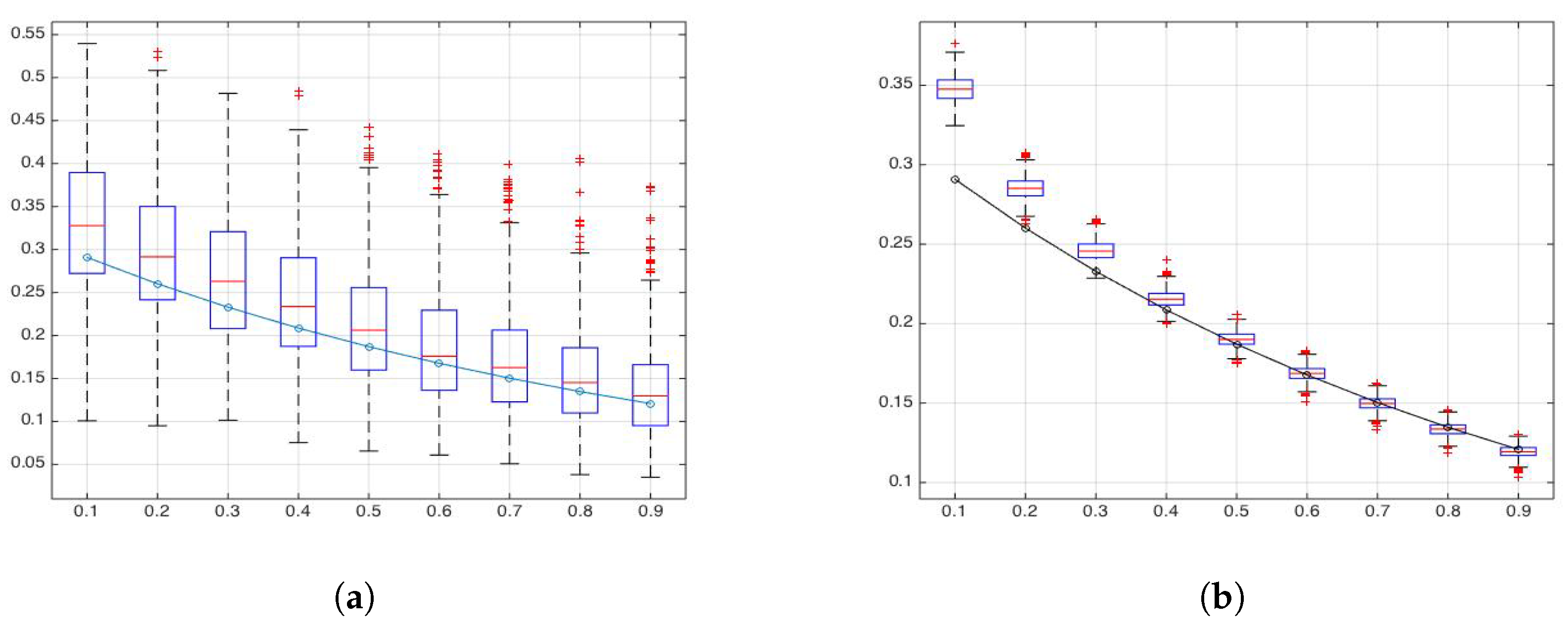
Results were similar to those obtained by [27] for the one-dimensional case: the wavelet-based estimator had good performance for $H>0.3$. In Figure 3, wavelet-based Shannon entropy measures are compared with the theoretical result of Equation (21) using $H=0.1,\dots ,0.9$. In particular, in Figure 3a, we used the empirical wavelet coefficients for estimating wavelet-based entropy, such as in Equation (10). In Figure 3b, we used the estimated Hurst parameters for estimating the wavelet-based Shannon entropy of Equation (21).

Although the variability of wavelet-based entropy was higher in the empirical case, median values were very close to the theoretical results. This result can be used for characterizing a 2D fractional Brownian field and describing its entropy.

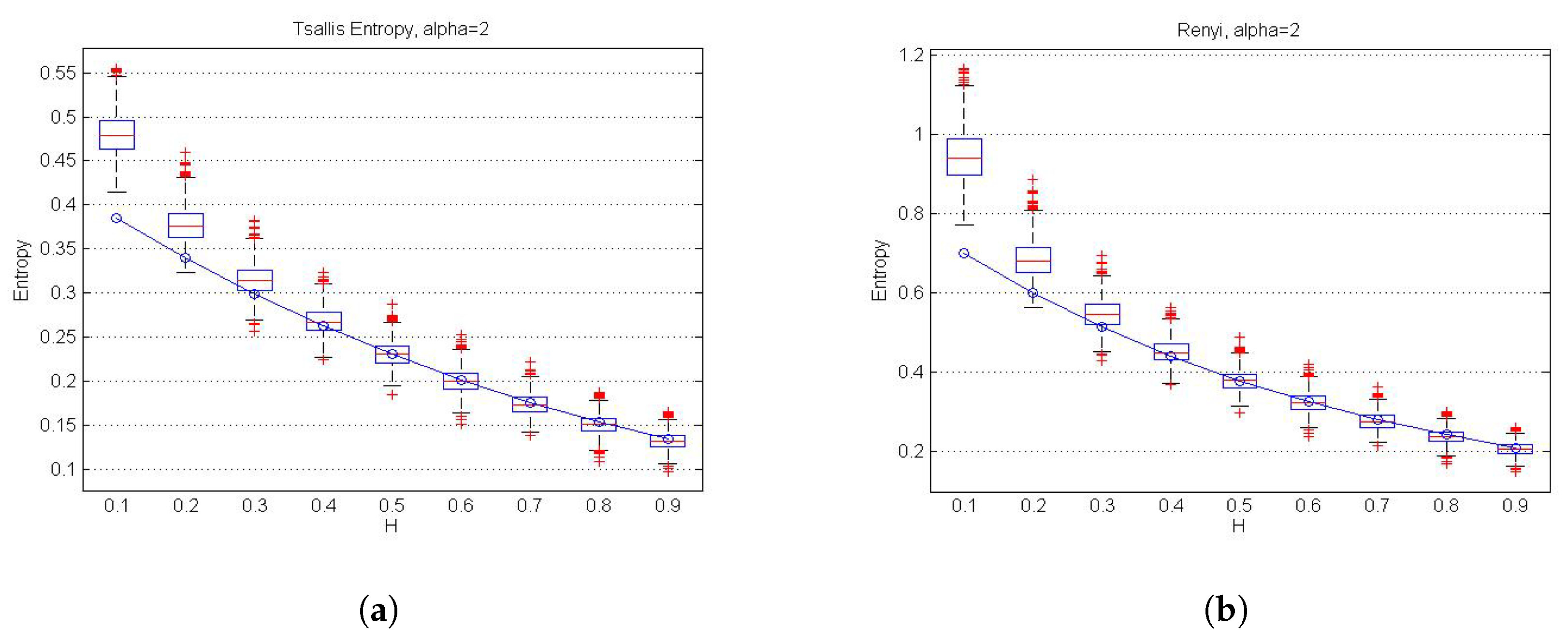
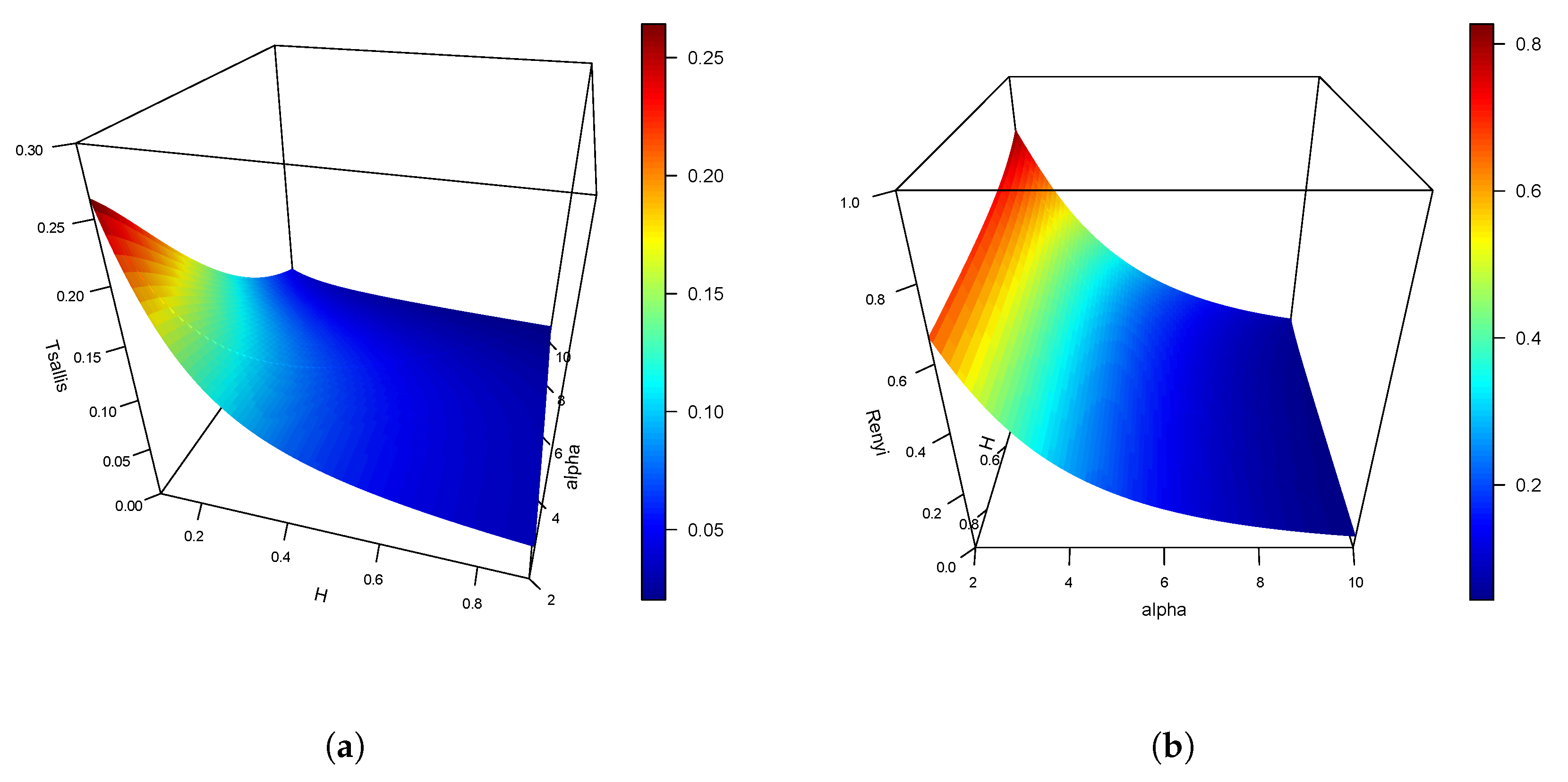
Additionally, we estimated wavelet-based Tsallis and Rényi (for $\alpha =2$) entropies for the simulated 2D fractional Brownian fields (Figure 4a,b, respectively) and we compared them with their theoretical values for each H (with $H=0.1,\dots ,0.9$). These plots show that Tsallis and Rényi entropies both decreased with higher values of H. However, more robust methods have to be used for estimating Hurst parameters when H is very small (for example, for $H=0.1$), since the wavelet method seems to underestimate real values, hence affecting the estimation of entropy measures. Since the result of this work allows to estimate entropy measures independently of the used wavelets, a different method could be used for estimating the Hurst parameter. In Figure 5a,b, we show the different behavior of Tsallis and Rényi entropies, respectively, for different values of $\alpha .$

6. Conclusions

In this work, we derived a mathematical expression for defining 2D Shannon, Tsallis, and Rényi entropies for a 2D fractional Brownian field. Results showed that the different proposed entropies are independent from the choice of wavelet function, allowing the use of different methods for estimating the Hurst parameter. The proposed formulations could be used in many applications where the generating process is a 2D fractional Brownian motion. Furthermore, these results could easily be extended to the $n-$ dimensional case. Some generalizations could also be considered for the study of anisotropic fractional Brownian fields by taking into account continuous wavelet transform, such as fully anisotropic wavelets introduced by [44] and successively used by [28]. Finally, our future steps are evaluating and validating these results on real datasets.

References

- Clausius, R. On the motive power of heat, and on the laws which may be deduced from it for the theory of heat. Annalen der Physick 1850, 368, 500. [Google Scholar] [CrossRef]
- Boltzmann, L. Einige allgemeine Satze iiber Warmegleichgewicht unter Gas- molekulen. Sitzungsber. Akad. Wiss. Wien 1871, 63, 679–711. [Google Scholar]
- Shannon, C. A mathematical theory of communication. Bell Syst. Technol. J. 1948, 27, 379–423. [Google Scholar] [CrossRef] [Green Version]
- Sengupta, B.; Stemmler, M.B.; Friston, K.J. Information and Efficiency in the Nervous System-A Synthesis. PLoS Comput. Biol. 2013, 9, e1003157. [Google Scholar] [CrossRef] [PubMed] [Green Version]
- Wong, A.K.C.; Sahoo, P.K. A gray level threshold selection method based on maximum entropy principle. IEEE Trans. Syst. Man Cyber. 1989, 19, 866–871. [Google Scholar] [CrossRef]
- Zhang, Y.; Wu, L. Optimal Multi-Level Thresholding Based on Maximum Tsallis Entropy via an Artificial Bee Colony Approach. Entropy 2011, 13, 841–859. [Google Scholar] [CrossRef] [Green Version]
- AghaKouchak, A. Entropy-Copula in Hydrology and Climatology. J. Hydrometeorol. 2014, 15, 2176–2189. [Google Scholar] [CrossRef]
- Koutsoyiannis, D. Uncertainty, entropy, scaling and hydrological stochastics. 2. Time dependence of hydrological processes and time scaling. Hydrol. Sci. J. 2005, 50, 405–426. [Google Scholar] [CrossRef]
- Li, S.; Zhou, Q.; Wu, S.; Dai, E. Measurement of climate complexity using sample entropy. Int. J. Clim. 2006, 26, 2131–2139. [Google Scholar]
- Oladipo, E.O. Spectral analysis of climatological time series: On the performance of periodogram, non-integer and maximum entropy methods. Theor. Appl. Clim. 1988, 39, 40–53. [Google Scholar] [CrossRef]
- Nicholson, T.; Sambridge, M.; Gudmundsson, O. On entropy and clustering in earthquake hypocentre distributions. Geophys. J. Int. 2000, 142, 37–51. [Google Scholar] [CrossRef] [Green Version]
- Telesca, L.; Lapenna, V.; Lovallo, M. Information entropy analysis of seismicity of Umbria-Marche region (Central Italy). Nat. Hazards Earth Syst. Sci. 2004, 4, 691–695. [Google Scholar] [CrossRef] [Green Version]
- Telesca, L.; Lovallo, M.; Mohamed, A.E.-E.A.; ElGabry, M.; El-hady, S.; Abou Elenean, K.M.; ElBary, R.E.F. Informational analysis of seismic sequences by applying the Fisher Information Measure and the Shannon entropy: An application to the 2004–2010 seismicity of Aswan area (Egypt). Physica A 2012, 391, 2889–2897. [Google Scholar] [CrossRef]
- Telesca, L.; Lovallo, M.; Babayev, G.; Kadirov, F. Spectral and informational analysis of seismicity: An application to the 1996–2012 seismicity of the Northern Caucasus-Azerbaijan part of the greater Caucasus-Kopet Dag region. Physica A 2013, 392, 6064–6078. [Google Scholar] [CrossRef]
- Telesca, L.; Lovallo, M.; Chamoli, A.; Dimri, V.P.; Srivastava, K. Fisher-Shannon analysis of seismograms of tsunamigenic and non-tsunamigenic earthquakes. Physica A 2013, 392, 3424–3429. [Google Scholar] [CrossRef]
- Rényi, A. On Measures of Entropy and Information. In Proceedings of the 4th Berkeley Symposium on Mathematics, Statistics and Probability; The Regents of the University of California: Berkeley, CA, USA, 1961; Volume 1, pp. 547–561. [Google Scholar]
- Contreras-Reyes, J.E. Rényi entropy and complexity measure for skew-gaussian distributions and related families. Physica A 2015, 433, 84–91. [Google Scholar] [CrossRef] [Green Version]
- Tsallis, C. Possible generalization of Boltzmann-Gibbs statistics. J. Stat. Phys. 1988, 52, 479–487. [Google Scholar] [CrossRef]
- Mariz, A.M. On the irreversible nature of the Tsallis and Renyi entropies. Phys. Lett. A 1992, 165, 409–411. [Google Scholar] [CrossRef]
- Labat, D. Recent advances in wavelet analyses: Part 1. A review of concepts. J. Hydrol. 2005, 314, 275–288. [Google Scholar] [CrossRef]
- Sello, S. Wavelet entropy and the multi-peaked structure of solar cycle maximum. New Astron. 2003, 8, 105–117. [Google Scholar] [CrossRef] [Green Version]
- Rosso, O.; Blanco, S.; Yordanowa, J.; Kolev, V.; Figliola, A.; Schürmann, M.; Başar, E. Wavelet entropy: A new tool for analysis of short duration brain electrical signals. J. Neurosci. Meth. 2001, 105, 65–75. [Google Scholar] [CrossRef]
- Lyubushin, A. Prognostic properties of low-frequency seismic noise. Nat. Sci. 2012, 4, 659–666. [Google Scholar] [CrossRef] [Green Version]
- Lyubushin, A. How soon would the next mega-earthquake occur in Japan? Nat. Sci. 2013, 5, 1–7. [Google Scholar] [CrossRef] [Green Version]
- Zunino, L.; Pérez, D.G.; Garavaglia, M.; Rosso, O.A. Characterization of laser propagation through turbulent media by quantifiers based on the wavelet transform. Fractals 2004, 12, 223–233. [Google Scholar] [CrossRef] [Green Version]
- Zunino, L.; Pérez, D.G.; Garavaglia, M.; Rosso, O.A. Wavelet entropy of stochastic processes. Physica A 2007, 379, 503–512. [Google Scholar] [CrossRef] [Green Version]
- Perez, D.G.; Zunino, L.; Garavaglia, M.; Rosso, O.A. Wavelet entropy and fractional Brownian motion time series. Physica A 2006, 365, 282–288. [Google Scholar] [CrossRef] [Green Version]
- Nicolis, O.; Mateu, J. 2D Anisotropic Wavelet Entropy with an Application to Earthquakes in Chile. Entropy 2015, 17, 4155–4172. [Google Scholar] [CrossRef] [Green Version]
- Perez, D.G.; Zunino, L.; Martin, M.T.; Garavaglia, M.; Plastino, A.; Rosso, O.A. Model-free stochastic processes studied with q-wavelet-based informational tools. Phys. Lett. A 2007, 364, 259–266. [Google Scholar] [CrossRef]
- Ramirez-Pacheco, J.; Rizo-Dominguez, L.; Trejo-Sanchez, J.A.; Cortez-Gonzalez, J. A nonextensive wavelet (q,q′)-entropy for 1/fα signals. Rev. Mex. Fis. 2016, 62, 229–234. [Google Scholar]
- Zunino, L.; Perez, D.G.; Kowalski, A.; Martin, M.T.; Garavaglia, M.; Plastino, A.; Rosso, O.A. Fractional Brownian motion, fractional Gaussian noise, and Tsallis permutation entropy. Physica A 2008, 387, 6057–6068. [Google Scholar] [CrossRef]
- Ramirez-Pacheco, J.; Torres Roman, D.; Toral Cruz, H. Distinguishing Stationary/Nonstationary Scaling Processes Using Wavelet Tsallis-Entropies. Math. Probl. Eng. 2012, 2012, 867042. [Google Scholar] [CrossRef]
- Ramírez-Pacheco, J.; Torres-Román, D.; Rizo-Dominguez, L.; Trejo-Sanchez, J.; Manzano-Pinzón, F. Wavelet Fisher’s information measure of 1 = fα signals. Entropy 2011, 13, 1648–1663. [Google Scholar] [CrossRef]
- Mandelbrot, B.B.; Van Ness, J.W. Fractional Brownian Motions, Fractional Noises and Applications. SIAM Rev. 1968, 10, 422–437. [Google Scholar] [CrossRef]
- Nicolis, O.; Ramirez, P.; Vidakovic, B. 2-D Wavelet-Based Spectra with Applications. Comput. Stat. Data Anal. 2011, 55, 738–751. [Google Scholar] [CrossRef]
- Qian, H.; Raymond, G.M.; Bassingthwaighte, J.B. On two-dimensional fractional Brownian motion and fractional Brownian random field. J. Phys. A. Math. Gen. 1998, 31, L527–L535. [Google Scholar] [CrossRef]
- Pesquet-Popescu, B.; Lèvy-Vèhel, J. Stochastic Fractal Models for Image Processing. IEEE Signal Proces. Mag. 2002, 19, 48–62. [Google Scholar] [CrossRef] [Green Version]
- Reed, I.S.; Lee, P.C.; Truong, T.K. Spectral representation of fractional Brownian motion in n dimensions and its properties. IEEE Trans. Inf. Theor. 1995, 41, 1439–1451. [Google Scholar] [CrossRef]
- Brouste, A.; Istas, J.; Lambert-Lacroix, S. On simulation of manifold indexed fractional gaussian fields. J. Stat. Soft. 2010, 34, 1–14. [Google Scholar] [CrossRef] [Green Version]
- Mallat, S. A Wavelet Tour of Signal Processing, 2nd ed.; Elsevier: Amsterdam, The Netherlands, 1999. [Google Scholar]
- Donoho, D.L. Nonlinear wavelet methods for recovery of signals, densities, and spectra from indirect and noisy data. In Different Perspectives on Wavelets; Daubechies, I., Ed.; American Mathematical Society: San Antonio, Texas, USA, 1993; pp. 173–205. [Google Scholar]
- Derado, G.; Lee, K.; Nicolis, O.; Bowman, F.D.; Newell, M.; Ruggeri, F.; Vidakovic, B. Wavelet-based 3-D Multifractal Spectrum with Applications in Breast MRI Images. In Bioinformatics Research and Applications; Lecture Notes in Computer Science; Springer: Berlin/Heidelberg, Germany, 2008; pp. 281–292. [Google Scholar]
- Heneghan, C.; Lown, S.B.; Teich, M.C. Two dimensional fractional Brownian motion: Wavelet analysis and synthesis. In Proceedings of the Southwest Symposium on Image Analysis and Interpretation, San Antonio, TX, USA, 8–9 April 1996; pp. 213–217. [Google Scholar]
- Neupauer, R.M.; Powell, K.L. A fully-anisotropic morlet wavelet to identify dominant orientations in a porous medium. Comput. Geosci. 2005, 13, 465–471. [Google Scholar] [CrossRef]
Figure 1.
Simulated fractional Brownian fields (fBf) using (a) and (b) .
Figure 2.
Boxplots of estimated Hurst parameter for each H parameter (). Dashed line, identity.
Figure 3.
(a) Boxplots of empirical wavelet-based Shannon wavelet entropy and (b) theoretical wavelet-based Shannon entropy using estimated Hurst parameters. Dashed line, theoretical wavelet Shannon entropy for .
Figure 4.
Boxplots of theoretical wavelet-based (a) Tsallis and (b) Rényi entropies using estimated Hurst parameters. Dashed line, theoretical Tsallis () and Rényi () entropies, respectively, for and .
Figure 5.
Theoretical wavelet-based (a) Tsallis and (b) Rényi entropies for , , and .
© 2020 by the authors. Licensee MDPI, Basel, Switzerland. This article is an open access article distributed under the terms and conditions of the Creative Commons Attribution (CC BY) license (http://creativecommons.org/licenses/by/4.0/).
Share and Cite
MDPI and ACS Style
Nicolis, O.; Mateu, J.; Contreras-Reyes, J.E. Wavelet-Based Entropy Measures to Characterize Two-Dimensional Fractional Brownian Fields. Entropy 2020, 22, 196. https://doi.org/10.3390/e22020196
AMA Style
Nicolis O, Mateu J, Contreras-Reyes JE. Wavelet-Based Entropy Measures to Characterize Two-Dimensional Fractional Brownian Fields. Entropy. 2020; 22(2):196. https://doi.org/10.3390/e22020196
Chicago/Turabian StyleNicolis, Orietta, Jorge Mateu, and Javier E. Contreras-Reyes. 2020. "Wavelet-Based Entropy Measures to Characterize Two-Dimensional Fractional Brownian Fields" Entropy 22, no. 2: 196. https://doi.org/10.3390/e22020196
Note that from the first issue of 2016, this journal uses article numbers instead of page numbers. See further details here.