Explicit Lump Solitary Wave of Certain Interesting (3+1)-Dimensional Waves in Physics via Some Recent Traveling Wave Methods


1
Department of Mathematics, Faculty of Science, Jiangsu University, Zhenjiang 212013, China
2
Department of Basic Science, Higher Technological Institute 10th of Ramadan City, El Sharqia 44634, Egypt
*
Authors to whom correspondence should be addressed.
Entropy 2019, 21(4), 397; https://doi.org/10.3390/e21040397
Submission received: 31 January 2019
/
Revised: 4 April 2019
/
Accepted: 4 April 2019
/
Published: 15 April 2019
(This article belongs to the Collection Wavelets, Fractals and Information Theory)
Abstract
:This study investigates the solitary wave solutions of the nonlinear fractional Jimbo–Miwa (JM) equation by using the conformable fractional derivative and some other distinct analytical techniques. The JM equation describes the certain interesting (3+1)-dimensional waves in physics. Moreover, it is considered as a second equation of the famous Painlev’e hierarchy of integrable systems. The fractional conformable derivatives properties were employed to convert it into an ordinary differential equation with an integer order to obtain many novel exact solutions of this model. The conformable fractional derivative is equivalent to the ordinary derivative for the functions that has continuous derivatives up to some desired order over some domain (smooth functions). The obtained solutions for each technique were characterized and compared to illustrate the similarities and differences between them. Profound solutions were concluded to be powerful, easy and effective on the nonlinear partial differential equation.
1. Introduction
During the last five decades, the nonlinear fractional partial differential equations (NLFPD) have been used for modeling many of the nonlinear phenomena in various fields. For instance, physics, chaos synchronization, continuous-time random walk, mechanical engineering, dynamical and sub-diffusive systems, anomalous diffusive, wave propagation phenomenon and so on. The non-local property is considered as the fundamental advantage of discovering many distinct properties of fractal models. Fractional calculus is a generalization of ordinary calculus, where derivatives and integrals of arbitrary real or complex order are defined. These fractional operators may model more efficiently certain real-world phenomena, especially when the dynamics are affected by constraints inherent to the system. According to the fundamental role of fractal models, an extensive study is applied on the fractional calculus to discover new fractional derivatives that have been defined such as the Riemann–Liouville, Caputo, Hadamard, Riesz, Grünwald–Letnikov, Marchaud, etc. [1,2,3,4,5]. These kinds of derivatives are linear operators and possess some fine properties, but they are not available for all other operational behaviors of a typical first derivative, such as chain rule, quotient rule, semigroup property, and product rule. Failure of previously mentioned derivatives created the interest of many researchers to derive a new derivative until, in 2014, R. Khalil et al. were discovered a new kind of derivative that is a new local fractional derivative which is well-behaved and complies with the computational relationships of the first derivative, called conformable derivative [6,7,8,9,10]. In the following steps, we give the summarized properties of this kind of derivative as follows:
For the given function , then the conformable derivatives of it with order where , is given by
for all . If f is -differentiable in , , and exists, then define
For classical definition of and Caputo on polynomial, we see the conformable derivative coincides with them such as it takes the following definition
where m is arbitrary constant.
For chain rule, quotient rule and semi group property, we see the properties of conformable derivative given by
where a and b are arbitrary constants.
where is arbitrary constant.
and also
when f is differentiable. According to these properties and definitions of conformable fractional derivative, it is equivalent to the ordinary derivative for smooth functions [11,12].
Definition 1.
The local fractional derivatives:
let be a continuous nonnegative map such that whenever Given a function and a real, we say that f is -differentiable at , with respect to kernel k, if the limit that given by Equation (1), exists. The derivative at is defined by
if the limit exists.
Consider the limit In this case, for , we obtain the classical definition of the fraction that is matched with conformable fractional derivative definition. Based on the conformable derivative definition, the fractional models convert to nonlinear ordinary differential equations with integer order. In this step, the contribution of both analytical and numerical schemes have started to study explicit solutions for these models and for this purpose, many analytical and approximate schemes have been derived such as exp -expansion, improved F-expansion, extended -expansion, extended tanh- function, simplest and extended simplest equation, generalized Riccati expansion and sinh-Gordon expansion, Riccati–Bernoulli Sub-ODE, and modified Khater methods to discover more physical and dynamical properties of these models. For further information about these methods, you can see [13,14,15,16,17,18,19,20,21,22,23,24,25,26,27].
This research applies a nine recent methods to the nonlinear time fractional Jimbo–Miwa (JM) equation for studying the properties of exact and solitary wave solutions. Moreover, we study the performance of a novel technique that has called the modified auxiliary equation method (modified Khater method) on the same model for examining the similarities and differences between these methods.
In 1983, Jimbo and Miwa put the structure of the JM model in the following formula [28]:
where describes a certain wave in physics. This model is the second equation in the well-known KP hierarchy of integrable systems that are given by [29]
where is a scalar function, represent longitudinal, transverse spatial coordinates, time, and arbitrary constant, respectively. However, it does not pass any of the conventional integrability tests. It is shown to be conditionally integrable having two types of solitary wave solutions such that the solitary waves in second type do not interact elastically. Equation (11) has two forms that depend on the values of as follows [30,31,32,33,34]:
The rest of the paper is organized as follows: Section 2 applies the above-mentioned techniques to the nonlinear time fractional JM equation to obtain exact and solitary wave solutions. Section 3 sketches some figures (Figure 1, Figure 2, Figure 3, Figure 4, Figure 5, Figure 6, Figure 7, Figure 8, Figure 9 and Figure 10) for the solutions and gives the physical interpretation of them. Section 4 gives a full discussion about the similarities and differences between these methods. Section 5 summaries the main conclusions.
2. Explicit Wave Solutions of the Nonlinear Time Fractional JM Model
This part tests the performance of ten analytical techniques on the nonlinear time fractional Jimbo–Miwa (JM). This model has a variety of solutions with distinct structures such as single-soliton solutions, multiple-soliton solutions, periodic wave solutions, and traveling wave solutions [37,38,39,40,41,42,43,44]. The fractional mathematical modeling of this equation is given as follows:
where describes the dynamics of a certain (3+1)-dimensional waves in physics and are arbitrary constants. Transformation the NLFPD equation into the NLPD equation with integer order by using the following conformable fractional derivative yields:
Calculating the homogeneous balance value between the highest order derivative and nonlinear terms of Equation (13) gives .
2.1. Utilization of Exp -Expansion Method
Applying this method enables putting the general solution of Equation (13) in the next formula:
where is arbitrary constant and is the solution function of the next ODE
where , and are arbitrary constants. Handling Equation (13) by utilizing Equation (14) and its derivatives, converts the left-hand side of Equation (13) to a polynomial equation of . Gathering all coefficients of term that has the same degree and equating them to zero. Solving the obtained algebraic system of equations leads to
According to the value of these parameters, we get the relevant traveling wave solutions of Equation (12):
When :
When :
When :
When :
When :
2.2. Utilization of the Improved F-Expansion Method
Applying this method enables putting the general solution of Equation (13) in the next formula:
where is arbitrary constant and is the solution of the next ODE
Handling of Equation (13) by utilizing Equation (22) and its derivatives converts the left-hand side of Equation (13) to a polynomial function of . Gather all coefficients of terms that have the same degree and equate them to zero. Solving the obtained system of equations yields.
Family I:
According to the value of these parameters, we get the relevant traveling wave solutions of Equation (12):
When :
When :
Family II:
According to the value of these parameters, we get the relevant traveling wave solutions of Equation (12):
When :
When :
2.3. Utilization of an Extended -Expansion Method
Applying this method enables putting the general solution of Equation (13) in the next formula:
where are arbitrary constants and is the solutions of the next ODE
where is arbitrary constant. Handling of Equation (13) by utilizing Equation (31) and its derivatives converts the left-hand side of Equation (13) to the polynomial function of where . Gather all coefficients of terms that have the same degree and equate them to zero. Solving the obtained system of equation yields
Family I:
According to the value of these parameters, the relevant traveling wave solutions of Equation (12) are given by the following formulas:
When :
When :
Family II:
According to the value of these parameters, the relevant traveling wave solutions of Equation (12) are given by the following formulas:
When :
When :
2.4. Utilization of an Extended Tanh-Function Method
Applying this method enables putting the general solution of Equation (13) into the next formula:
where and is the solution of the next ODE
where d is arbitrary constants. Handling of Equation (13) by utilizing Equation (36) and its derivatives converts the left-hand side of Equation (13) to polynomial function of . Gather all coefficients of terms that have a same degree and equate them to zero. Solving the obtained system of equation results in
Family I:
According to the value of these parameters, the relevant traveling wave solutions of Equation (12) are given by the following formulas:
When :
When :
When :
Family II:
According to the value of these parameters, the relevant traveling wave solutions of Equation (12) are given by the next formulas:
When :
When :
When :
Family III:
According to the value of these parameters, the relevant traveling wave solutions of Equation (12) are given by the following formulas:
When :
When :
2.5. Utilization of the Simplest Equation Method
Applying this method enables putting the general solution of Equation (13) in the next formula:
where is arbitrary constant and is the solutions of the next ODE
where are arbitrary constants. Handling of Equation (13) by utilizing Equation (49) and its derivatives converts the left-hand side of Equation (13) to polynomial function of . Gathering all coefficients of terms that have the same degree and equating them to zero. Solving the obtained system of equation obtains
Family I
According to the value of these parameters, the relevant traveling wave solutions of Equation (12) are given as follows:
When :
Family II
According to the value of these parameters, the relevant traveling wave solutions of Equation (12) are given as follows:
When :
2.6. Utilization of an Extended Simplest Equation Method
Applying this method enables putting the general solution of Equation (13) in the next formula:
where and is the solution of the next ODE
where are arbitrary constants. Handling Equation (13) by utilizing Equation (53) and its derivatives converts the left-hand side of Equation (13) to polynomial function of . Gather all coefficients of terms that have the same degree and equate them to zero. Solving the obtained system of equation, we get:
Family I
According to the value of these parameters, the relevant traveling wave solutions of Equation (12) are given as follows:
When :
Thus, when the solutions take the following forms:
When :
When :
Thus, when the solutions take the following forms:
When : while :
When :
Thus, when the solutions take the following forms:
Family II
According to the value of these parameters, the relevant traveling wave solutions of Equation (12) are given as follows:
When :
While :
While :
When :
Thus, when the solutions take the following forms:
When :
While :
2.7. Utilization of the Generalized Riccati Expansion Method
Applying this method enables putting the general solution of Equation (13) in the next formula:
where and is the solution of the next ODE
where are arbitrary constants. Handling of Equation (13) by utilizing Equation (72) converts the left-hand side of Equation (13) to polynomial function of . Gather all coefficients of terms that have the same degree and equate them to zero. Solving the obtained system of equation leads to
According to the value of these parameters, we get the relevant traveling wave solutions of Equation (12):
When :
When :
2.8. Utilization of the Generalized Sinh–Gordon Expansion Method
Applying this method enables putting the general solution of Equation (13) in the next formula:
where are arbitrary constants. Handling of Equation (13) by utilizing Equation (97) and its derivatives converts the left-hand side of Equation (13) to polynomial function of . Gather all coefficients of terms that have the same degree and equate them to zero. Solving the obtained system of equation leads to
Case I: When :
Family I:
According to the value of these parameters, the relevant traveling wave solutions of Equation (12) are given in the following formulas:
Family II:
According to the value of these parameters, the relevant traveling wave solutions of Equation (12) are given in the following formulas:
Case II: When :
Family I:
According to the value of these parameters, the relevant traveling wave solutions of Equation (12) are given by the following formulas:
2.9. Utilization of Riccati–Bernoulli Sub-ODE Method
Applying this method enables putting the general solution of Equation (13) in the next formula:
where are arbitrary constants. Substituting Equation (104) and its derivatives into Equation (13), in addition to collecting all coefficients of the same term of , we get the system of equation. Solving this system leads to
Family I:
Thus, the solitary wave solutions of Equation (12) are given by
When
When
2.10. Utilization of the Modified Auxiliary Method
Applying this method enables putting the general solution of Equation (13) in the next formula:
where are arbitrary constants and is the solution of the next ODE
where are arbitrary constants. Handling of Equation (13) by utilizing Equation (111) and its derivatives converts the left-hand side of Equation (13) to polynomial function of . Gather all coefficients of terms that have the same degree and equate them to zero. Solving the obtained system of equation yields:
Family I:
According to the value of these parameters, the relevant traveling wave solutions of Equation (12) are given as follows:
When :
When :
When :
When :
When :
When :
When :
When :
When :
When :
When :
When :
When :
When :
Family II:
According to the value of these parameters, the relevant traveling wave solutions of Equation (12) are given as follows:
When :
When :
When :
When :
When :
When :
When :
When :
When :
When :
When :
When :
When :
When :
3. Physical Interpretation of Solution
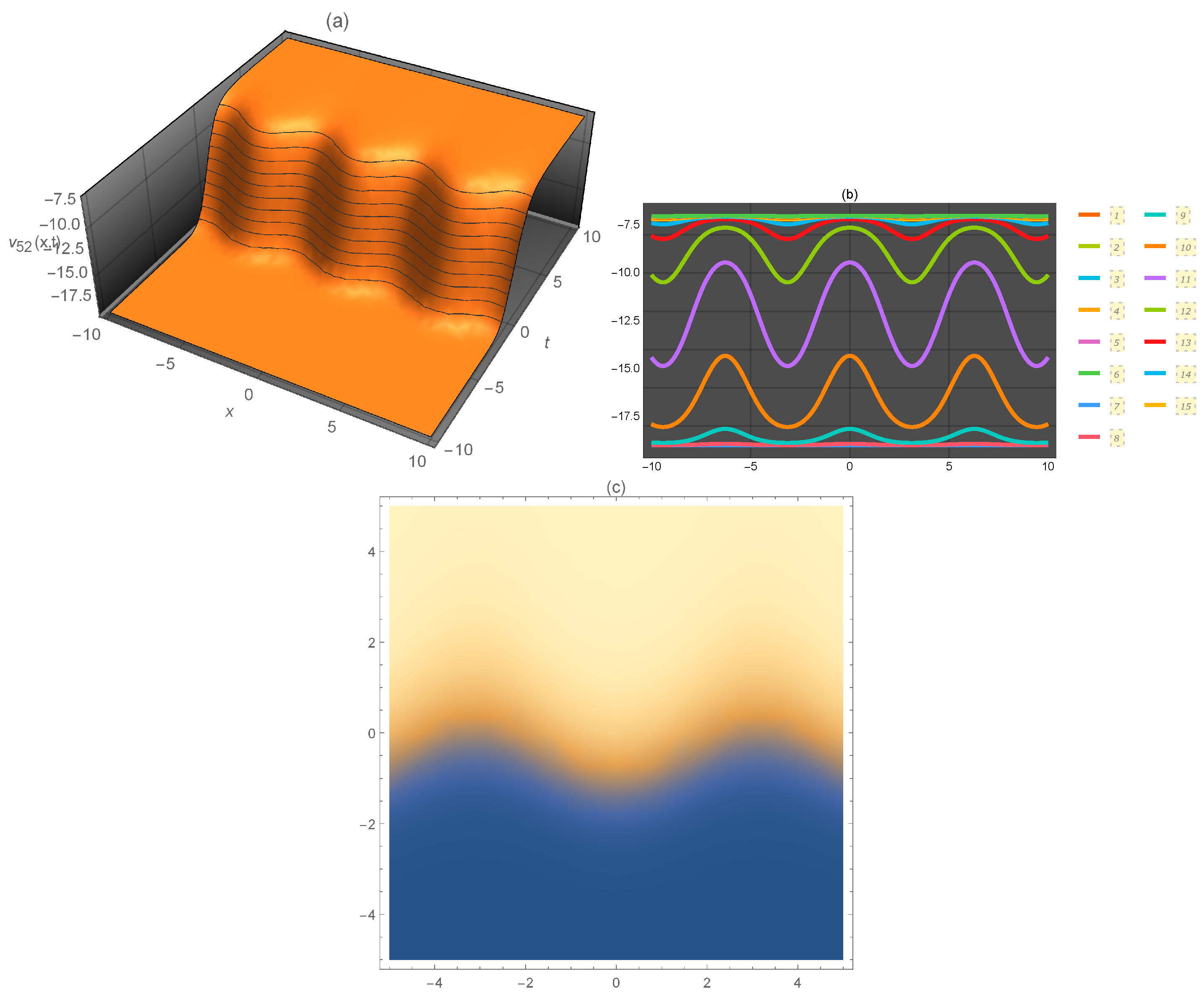
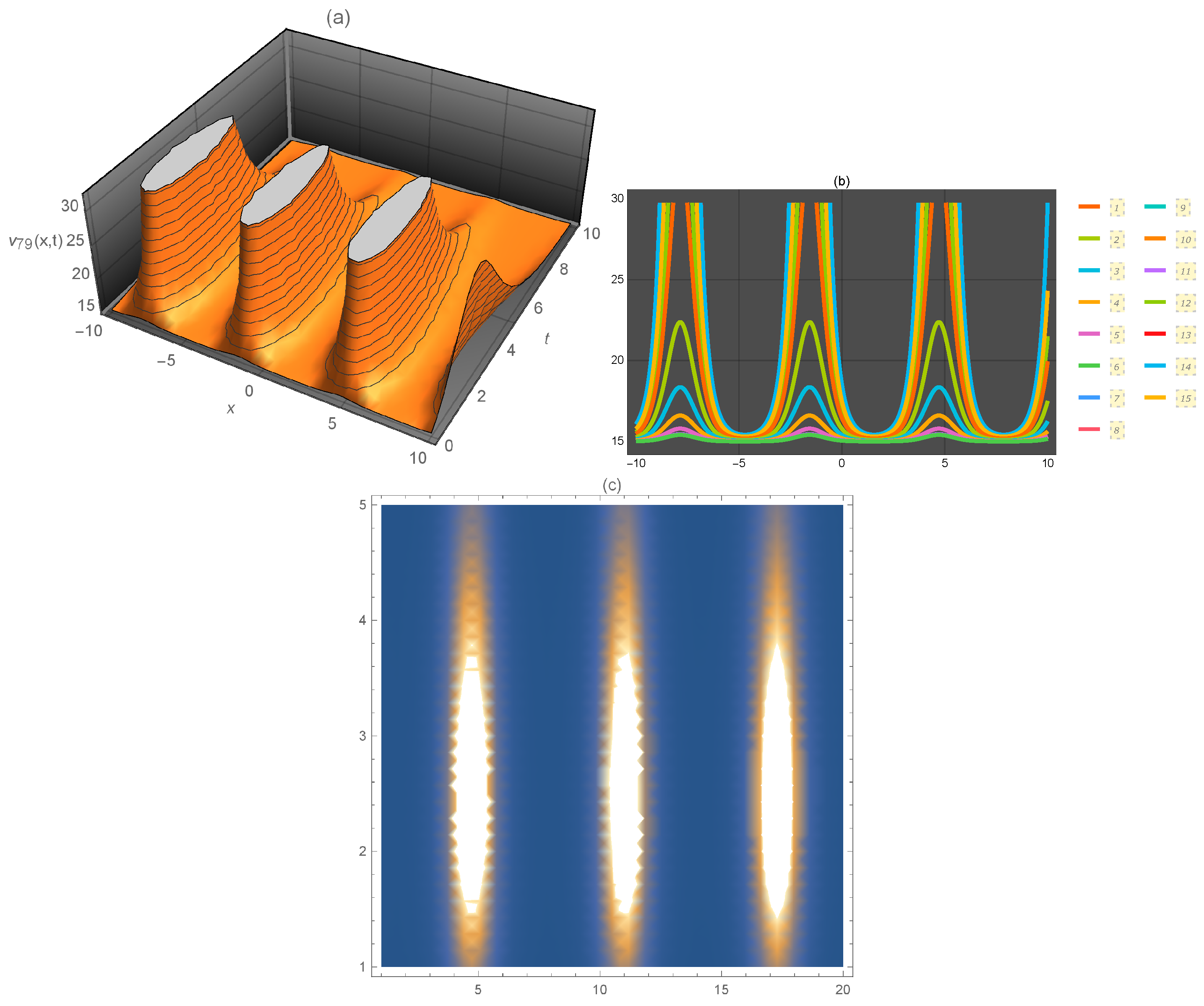
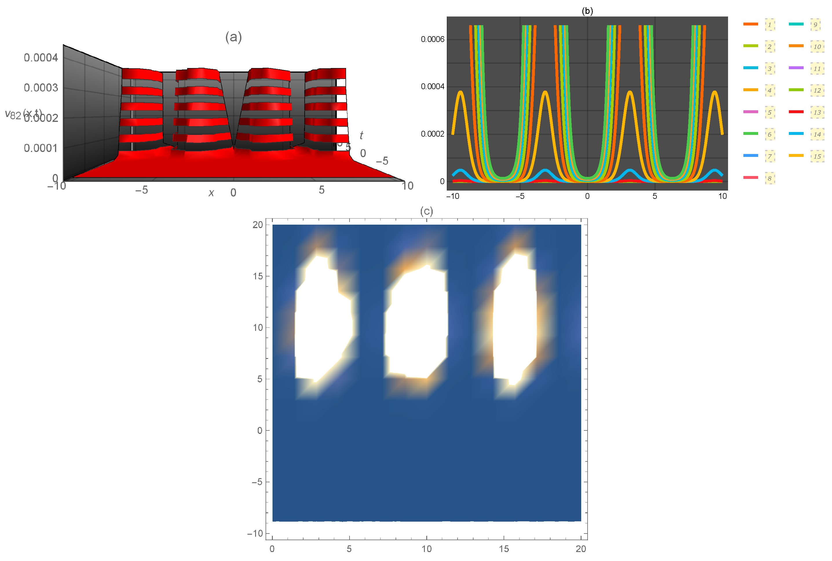
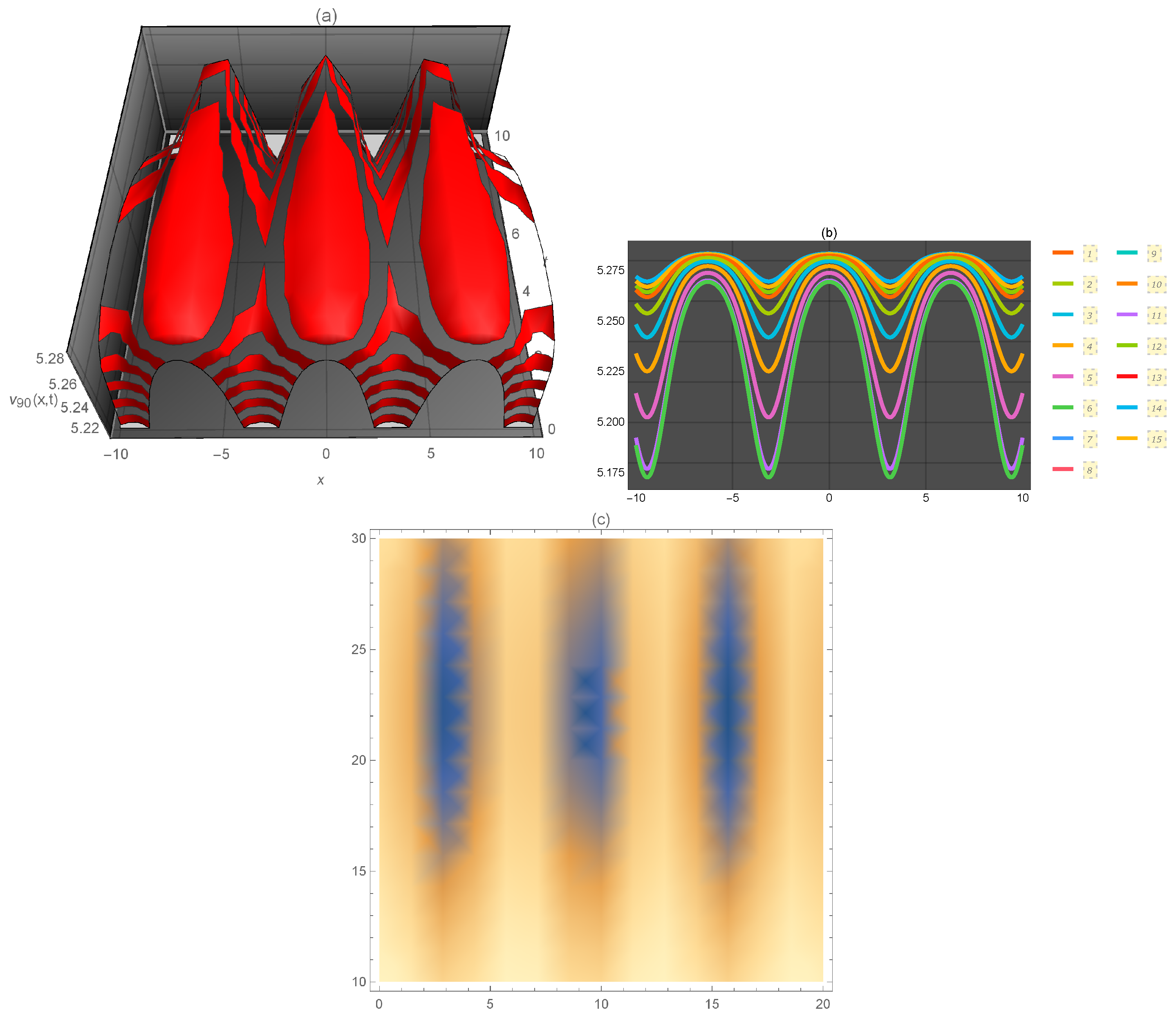
This section discusses and interprets some of the obtained solutions under the suitable choice of the parameters values as shown in Table 1. Generally, all of these waves are considered as traveling from right to left.
4. Discussion
This section investigates the relation between all above-mentioned methods with a modified auxiliary equation method (modified Khater method). We show the similarities and differences between them and the result of this discussion is shown in Table 2.
According to this discussion, we can conclude that the modified auxiliary equation method (modfied Khater method) covers the first seven methods that are used in this research and it is more general than them.
5. Conclusions
This paper studied the performance of conformable fractional derivative on the time fractional Jimbo–Miwa equation. Moreover, nine analytical and modified auxiliary equation methods (modified Khater method) were applied to this model for getting various explicit wave solutions of the fractional JM model. The solutions obtained were discussed and represented under the suitable choice of the parameters to show the physical properties of each one of them. In addition, we studied each one of the used methods and its relation with the modified auxiliary equation method. Our discussion shows the superiority of the modified auxiliary equation method (modified Khater method) on some of these methods such that it covers almost all solutions that are obtained by these methods.
Author Contributions
M.M.A.K., D.L., and R.A.M.A. contributed to the design and implementation of the research, to the analysis of the results, and to the writing of the manuscript.
Funding
We did not receive any specific grant from any funding agency.
Acknowledgments
(Corresponding author: Mostafa M. A. Khater) I would like to dedicate this article to my mother, the soul of my father, my wife, and my son (Adam).
Conflicts of Interest
The authors declare no conflict of interest.
References
- Atangana, A.; Gómez-Aguilar, J. Numerical approximation of Riemann-Liouville definition of fractional derivative: From Riemann-Liouville to Atangana-Baleanu. Numer. Methods Partial Differ. Equ. 2018, 34, 1502–1523. [Google Scholar] [CrossRef]
- Owolabi, K.M. Mathematical analysis and numerical simulation of chaotic noninteger order differential systems with Riemann-Liouville derivative. Numer. Methods Partial Differ. Equ. 2018, 34, 274–295. [Google Scholar] [CrossRef]
- Zhang, H.; Ye, R.; Cao, J.; Alsaedi, A. Delay-independent stability of Riemann–Liouville fractional neutral-type delayed neural networks. Neural Process. Lett. 2018, 47, 427–442. [Google Scholar] [CrossRef]
- Li, L.; Liu, J.G. A generalized definition of Caputo derivatives and its application to fractional ODEs. SIAM J. Math. Anal. 2018, 50, 2867–2900. [Google Scholar] [CrossRef]
- Kumar, K.; Pandey, R.K.; Sharma, S. Approximations of fractional integrals and Caputo derivatives with application in solving Abel’s integral equations. J. King Saud Univ.-Sci. 2018, in press. [Google Scholar] [CrossRef]
- Abdeljawad, T.; Al-Mdallal, Q.M.; Jarad, F. Fractional logistic models in the frame of fractional operators generated by conformable derivatives. Chaos Solitons Fractals 2019, 119, 94–101. [Google Scholar] [CrossRef]
- Zhou, H.; Yang, S.; Zhang, S. Conformable derivative approach to anomalous diffusion. Phys. Stat. Mech. Its Appl. 2018, 491, 1001–1013. [Google Scholar] [CrossRef]
- Yang, S.; Wang, L.; Zhang, S. Conformable derivative: Application to non-Darcian flow in low-permeability porous media. Appl. Math. Lett. 2018, 79, 105–110. [Google Scholar] [CrossRef]
- Anderson, D.R.; Camrud, E.; Ulness, D.J. On the nature of the conformable derivative and its applications to physics. arXiv, 2018; arXiv:1810.02005. [Google Scholar]
- Abdelhakim, A.A.; Machado, J.A.T. A critical analysis of the conformable derivative. Nonlinear Dyn. 2019, 1–11. [Google Scholar] [CrossRef]
- Almeida, R.; Guzowska, M.; Odzijewicz, T. A remark on local fractional calculus and ordinary derivatives. Open Math. 2016, 14, 1122–1124. [Google Scholar] [CrossRef] [Green Version]
- Prodanov, D. Conditions for continuity of fractional velocity and existence of fractional Taylor expansions. Chaos Solitons Fractals 2017, 102, 236–244. [Google Scholar] [CrossRef]
- Attia, R.A.; Lu, D.; Khater, M.M.; Abd elazeem, O.M. Structure of New Solitary Solutions for The Schwarzian Korteweg De Vries Equation and (2+1)-Ablowitz-Kaup-Newell-Segur Equation. Phys. J. 2018, 1, 234–254. [Google Scholar]
- Khater, M.; Attia, R.; Lu, D. Modified Auxiliary Equation Method versus Three Nonlinear Fractional Biological Models in Present Explicit Wave Solutions. Math. Comput. Appl. 2019, 24, 1. [Google Scholar] [CrossRef]
- Khater, M.M.; Lu, D.; Attia, R.A. Dispersive long wave of nonlinear fractional Wu-Zhang system via a modified auxiliary equation method. AIP Adv. 2019, 9, 025003. [Google Scholar] [CrossRef]
- Attia, R.A.; Lu, D.; MA Khater, M. Chaos and Relativistic Energy-Momentum of the Nonlinear Time Fractional Duffing Equation. Math. Comput. Appl. 2019, 24, 10. [Google Scholar] [CrossRef]
- Biswas, A.; Mirzazadeh, M.; Triki, H.; Zhou, Q.; Ullah, M.Z.; Moshokoa, S.P.; Belic, M. Perturbed resonant 1-soliton solution with anti-cubic nonlinearity by Riccati-Bernoulli sub-ODE method. Optik 2018, 156, 346–350. [Google Scholar] [CrossRef]
- Kaur, B.; Gupta, R. Dispersion analysis and improved F-expansion method for space–time fractional differential equations. Nonlinear Dyn. 2019, 1–16. [Google Scholar] [CrossRef]
- Islam, M.S.; Akbar, M.A.; Khan, K. Analytical solutions of nonlinear Klein–Gordon equation using the improved F-expansion method. Opt. Quantum Electron. 2018, 50, 224. [Google Scholar] [CrossRef]
- Pandir, Y.; Duzgun, H.H. New exact solutions of the space-time fractional cubic Schrodinger equation using the new type F-expansion method. Waves Random Complex Media 2018, 1–10. [Google Scholar] [CrossRef]
- Liu, X.Z.; Yu, J.; Lou, Z.M.; Cao, Q.J. Residual Symmetry Reduction and Consistent Riccati Expansion of the Generalized Kaup-Kupershmidt Equation. Commun. Theor. Phys. 2018, 69, 625. [Google Scholar] [CrossRef]
- Raza, N.; Abdullah, M.; Butt, A.R.; Murtaza, I.G.; Sial, S. New exact periodic elliptic wave solutions for extended quantum Zakharov–Kuznetsov equation. Opt. Quantum Electron. 2018, 50, 177. [Google Scholar] [CrossRef]
- Shahoot, A.; Alurrfi, K.; Hassan, I.; Almsri, A. Solitons and other exact solutions for two nonlinear PDEs in mathematical physics using the generalized projective Riccati equations method. Adv. Math. Phys. 2018, 2018, 6870310. [Google Scholar] [CrossRef]
- Rezazadeh, H.; Korkmaz, A.; Eslami, M.; Vahidi, J.; Asghari, R. Traveling wave solution of conformable fractional generalized reaction Duffing model by generalized projective Riccati equation method. Opt. Quantum Electron. 2018, 50, 150. [Google Scholar] [CrossRef]
- El-Horbaty, M.; Ahmed, F. The Solitary Travelling Wave Solutions of Some Nonlinear Partial Differential Equations Using the Modified Extended Tanh Function Method with Riccati Equation. Asian Res. J. Math. 2018, 1–13. [Google Scholar] [CrossRef]
- Tian, Y. Quasi hyperbolic function expansion method and tanh-function method for solving vibrating string equation and elastic rod equation. J. Low Freq. Noise Vib. Act. Control 2019. [Google Scholar] [CrossRef]
- Pandir, Y.; Yildirim, A. Analytical approach for the fractional differential equations by using the extended tanh method. Waves Random Complex Media 2018, 28, 399–410. [Google Scholar] [CrossRef]
- Jimbo, M.; Miwa, T. Solitons and infinite dimensional Lie algebras. Publ. Res. Inst. Math. Sci. 1983, 19, 943–1001. [Google Scholar] [CrossRef]
- Kac, V.G.; van de Leur, J.W. The n-component KP hierarchy and representation theory. J. Math. Phys. 2003, 44, 3245–3293. [Google Scholar] [CrossRef]
- Zograf, P. Enumeration of Grothendieck’s dessins and KP hierarchy. Int. Math. Res. Not. 2015, 2015, 13533–13544. [Google Scholar] [CrossRef]
- Li, C.; Cheng, J.; Tian, K.; Li, M.; He, J. Ghost symmetry of the discrete KP hierarchy. Monatsh. Math. 2016, 180, 815–832. [Google Scholar] [CrossRef]
- Chalykh, O.; Silantyev, A. KP hierarchy for the cyclic quiver. J. Math. Phys. 2017, 58, 071702. [Google Scholar] [CrossRef] [Green Version]
- Kodama, Y. Lax-Sato Formulation of the KP Hierarchy. In KP Solitons and the Grassmannians; Springer: Berlin/Heidelberg, Germany, 2017; pp. 25–40. [Google Scholar]
- Nakayashiki, A. Degeneration of trigonal curves and solutions of the KP-hierarchy. Nonlinearity 2018, 31, 3567. [Google Scholar] [CrossRef]
- Gaillard, P. Rational solutions to the KPI equation and multi rogue waves. Ann. Phys. 2016, 367, 1–5. [Google Scholar] [CrossRef]
- Boiti, M.; Pempinelli, F.; Pogrebkov, A. KPII: Cauchy–Jost function, Darboux transformations and totally nonnegative matrices. J. Phys. Math. Theor. 2017, 50, 304001. [Google Scholar] [CrossRef] [Green Version]
- Korkmaz, A. Exact solutions to (3+1) conformable time fractional Jimbo–Miwa, Zakharov–Kuznetsov and modified Zakharov–Kuznetsov equations. Commun. Theor. Phys. 2017, 67, 479. [Google Scholar] [CrossRef]
- Aksoy, E.; Guner, O.; Bekir, A.; Cevikel, A.C. Exact solutions of the (3+1)-dimensional space-time fractional Jimbo-Miwa equation. AIP Conf. Proc. 2016, 1738, 290014. [Google Scholar]
- Kaplan, M.; Bekir, A. Construction of exact solutions to the space–time fractional differential equations via new approach. Optik 2017, 132, 1–8. [Google Scholar] [CrossRef]
- Ali, K.K.; Nuruddeen, R.; Hadhoud, A.R. New exact solitary wave solutions for the extended (3+1)-dimensional Jimbo-Miwa equations. Results Phys. 2018, 9, 12–16. [Google Scholar] [CrossRef]
- Korkmaz, A.; Hepson, O.E. Traveling waves in rational expressions of exponential functions to the conformable time fractional Jimbo–Miwa and Zakharov–Kuznetsov equations. Opt. Quantum Electron. 2018, 50, 42. [Google Scholar] [CrossRef] [Green Version]
- Sirisubtawee, S.; Koonprasert, S.; Khaopant, C.; Porka, W. Two Reliable Methods for Solving the (3+1)-Dimensional Space-Time Fractional Jimbo-Miwa Equation. Math. Probl. Eng. 2017, 2017, 9257019. [Google Scholar] [CrossRef]
- Kumar, D.; Seadawy, A.R.; Joardar, A.K. Modified Kudryashov method via new exact solutions for some conformable fractional differential equations arising in mathematical biology. Chin. J. Phys. 2018, 56, 75–85. [Google Scholar] [CrossRef]
- Zhang, J.-F.; Wu, F.-M. Bäcklund transformation and multiple soliton solutions for the (3+1)-dimensional Jimbo-Miwa equation. Chin. Phys. 2002, 11, 425. [Google Scholar]
Figure 1.
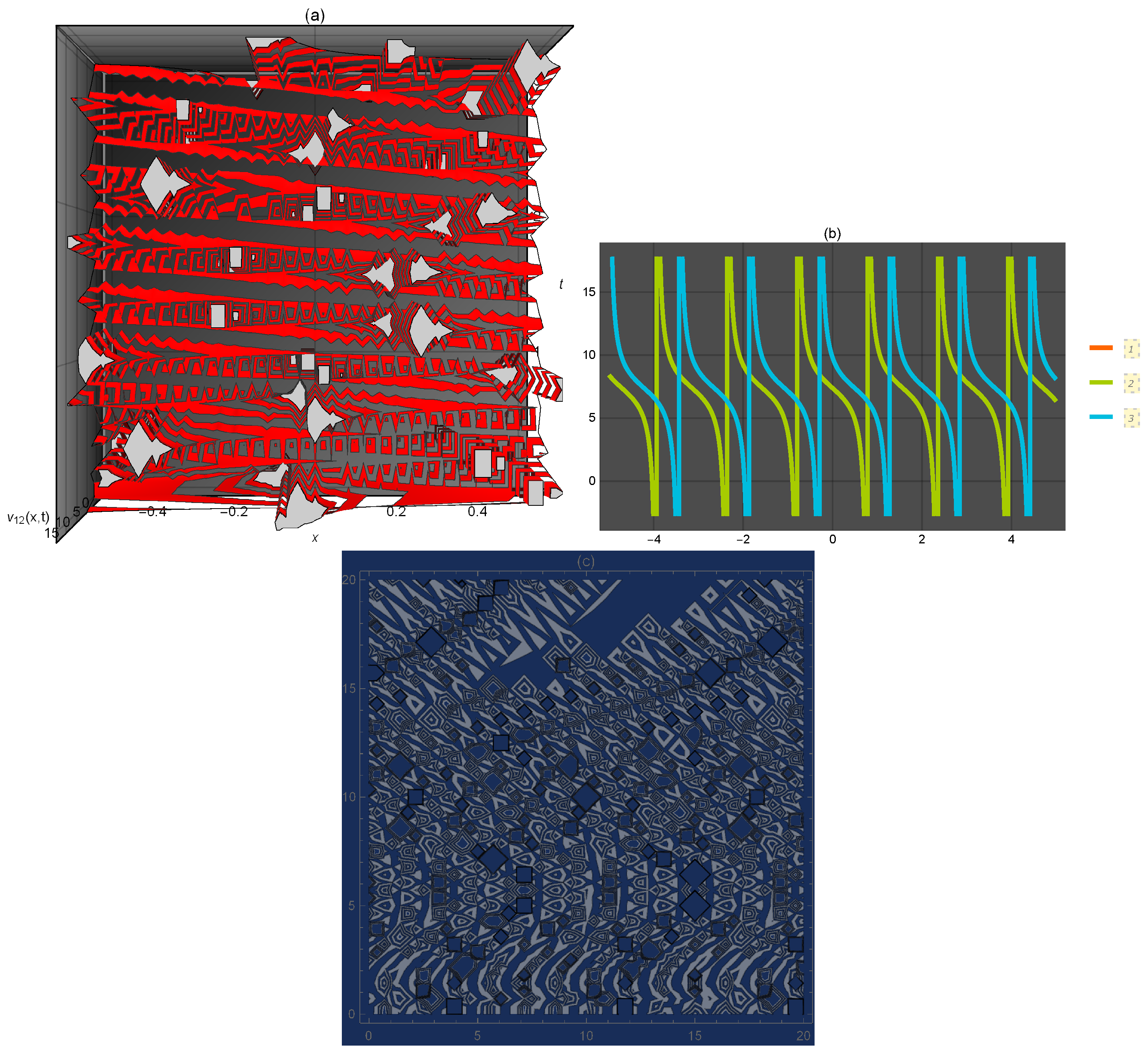
Representation of the solution of Equation (15): (a) three-dimensional ; (b) for several values of t and (c) density plot .
Figure 1.
Representation of the solution of Equation (15): (a) three-dimensional ; (b) for several values of t and (c) density plot .

Figure 2.
Representation of the solution of Equation (27): (a) three-dimensional ; (b) for several values of t and (c) density plot .
Figure 2.
Representation of the solution of Equation (27): (a) three-dimensional ; (b) for several values of t and (c) density plot .

Figure 3.
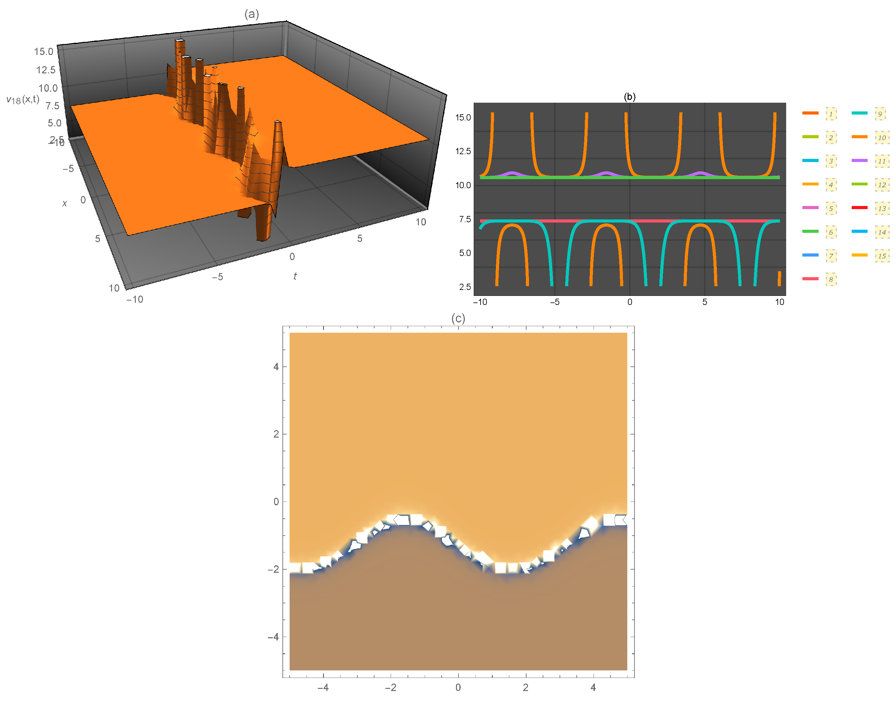
Representation of the solution of Equation (35): (a) three-dimensional ; (b) for several values of t and (c) density plot .
Figure 3.
Representation of the solution of Equation (35): (a) three-dimensional ; (b) for several values of t and (c) density plot .

Figure 4.
Representation of the solution of Equation (45): (a) three-dimensional ; (b) for several values of t and (c) density plot .
Figure 4.
Representation of the solution of Equation (45): (a) three-dimensional ; (b) for several values of t and (c) density plot .

Figure 5.
Representation of the solution of Equation (52): (a) three-dimensional ; (b) for several values of t and (c) density plot .
Figure 5.
Representation of the solution of Equation (52): (a) three-dimensional ; (b) for several values of t and (c) density plot .

Figure 6.
Representation of the solution of Equation (58): (a) three-dimensional ; (b) for several values of t and (c) density plot .
Figure 6.
Representation of the solution of Equation (58): (a) three-dimensional ; (b) for several values of t and (c) density plot .

Figure 7.
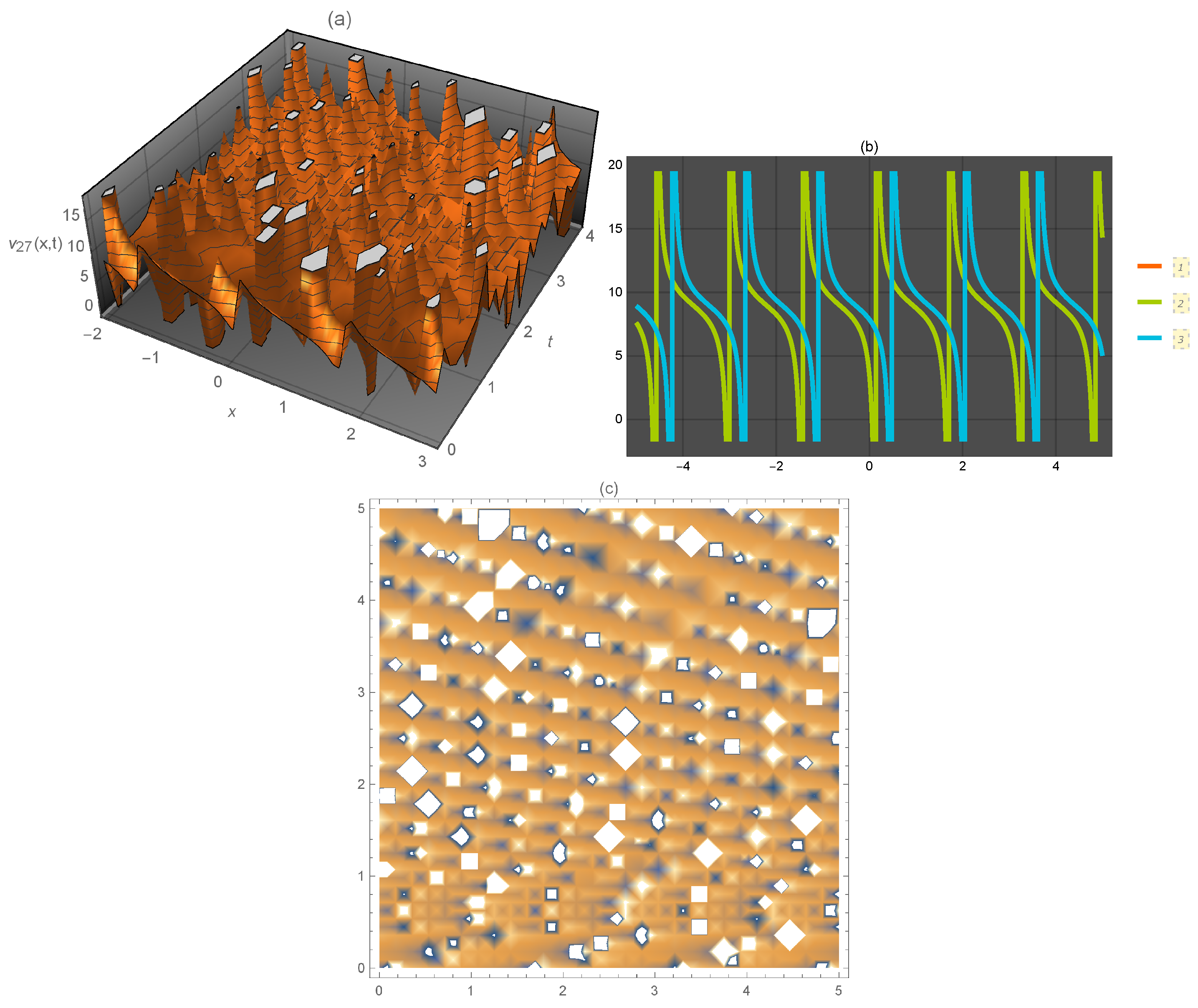
Representation of the solution of Equation (73): (a) three-dimensional ; (b) for several values of t and (c) density plot .
Figure 7.
Representation of the solution of Equation (73): (a) three-dimensional ; (b) for several values of t and (c) density plot .

Figure 8.
Representation of the solution of Equation (101): (a) three-dimensional ; (b) for several values of t and (c) density plot .
Figure 8.
Representation of the solution of Equation (101): (a) three-dimensional ; (b) for several values of t and (c) density plot .

Figure 9.
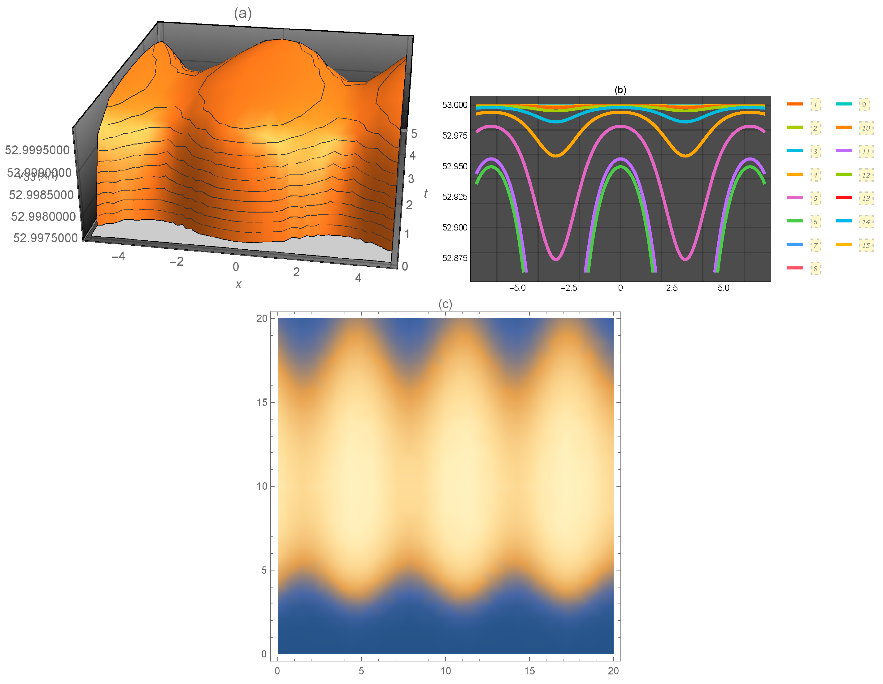
Representation of the solution of Equation (105): (a) three-dimensional ; (b) for several values of t and (c) density plot .
Figure 9.
Representation of the solution of Equation (105): (a) three-dimensional ; (b) for several values of t and (c) density plot .

Figure 10.
Representation of the solution of Equation (114): (a) three-dimensional ; (b) for several values of t and (c) density plot .
Figure 10.
Representation of the solution of Equation (114): (a) three-dimensional ; (b) for several values of t and (c) density plot .


Table 1.
Physical interpretation of represented solutions where represent shape, amplitude, and wavelength, respectively.
Table 1.
Physical interpretation of represented solutions where represent shape, amplitude, and wavelength, respectively.
| Fig. Nu. | S | A | W | Parameters Value |
|---|---|---|---|---|
| Periodic kink | 7.4 | 6 | ||
| Singular | 15 | 0.5 | ||
| Singular kink | 15 | 7 | ||
| Singular | 20 | 1.9 | ||
| Periodic kink | 1.2 | 0.7 | ||
| periodic kink | 53 | 7 | ||
| Kink | 10 | 6 | ||
| periodic anti-kink | 15 | 6 | ||
| periodic kink | 0.0006 | 6 | ||
| periodic kink | 0.1 | 6.5 |
Table 2.
Discussion of the relations between the modified auxiliary equation and above-mentioned methods.
Table 2.
Discussion of the relations between the modified auxiliary equation and above-mentioned methods.
| Method | Conditions | Similar |
|---|---|---|
| Exp -expansion method | √ | |
| Improved F-expansion method | √ | |
| Extended -expansion method | √ | |
| Extended tanh- function method | √ | |
| Simplest equation method | √ | |
| Extended simplest equation method | √ | |
| Generalized Riccati expansion method | √ | |
| Generalized Sinh–Gordon expansion method | x | |
| Riccati–Bernoulli Sub-ODE method | x |
© 2019 by the authors. Licensee MDPI, Basel, Switzerland. This article is an open access article distributed under the terms and conditions of the Creative Commons Attribution (CC BY) license (http://creativecommons.org/licenses/by/4.0/).
Share and Cite
MDPI and ACS Style
Khater, M.M.A.; Attia, R.A.M.; Lu, D. Explicit Lump Solitary Wave of Certain Interesting (3+1)-Dimensional Waves in Physics via Some Recent Traveling Wave Methods. Entropy 2019, 21, 397. https://doi.org/10.3390/e21040397
AMA Style
Khater MMA, Attia RAM, Lu D. Explicit Lump Solitary Wave of Certain Interesting (3+1)-Dimensional Waves in Physics via Some Recent Traveling Wave Methods. Entropy. 2019; 21(4):397. https://doi.org/10.3390/e21040397
Chicago/Turabian StyleKhater, Mostafa M. A., Raghda A. M. Attia, and Dianchen Lu. 2019. "Explicit Lump Solitary Wave of Certain Interesting (3+1)-Dimensional Waves in Physics via Some Recent Traveling Wave Methods" Entropy 21, no. 4: 397. https://doi.org/10.3390/e21040397
Note that from the first issue of 2016, this journal uses article numbers instead of page numbers. See further details here.