
When the Map Is Better Than the Territory

Department of Biological Sciences, Columbia University, New York, NY 10027, USA
Entropy 2017, 19(5), 188; https://doi.org/10.3390/e19050188
Submission received: 13 March 2017
/
Revised: 17 April 2017
/
Accepted: 21 April 2017
/
Published: 26 April 2017
(This article belongs to the Section Complexity)
Abstract
:The causal structure of any system can be analyzed at a multitude of spatial and temporal scales. It has long been thought that while higher scale (macro) descriptions may be useful to observers, they are at best a compressed description and at worse leave out critical information and causal relationships. However, recent research applying information theory to causal analysis has shown that the causal structure of some systems can actually come into focus and be more informative at a macroscale. That is, a macroscale description of a system (a map) can be more informative than a fully detailed microscale description of the system (the territory). This has been called “causal emergence.” While causal emergence may at first seem counterintuitive, this paper grounds the phenomenon in a classic concept from information theory: Shannon’s discovery of the channel capacity. I argue that systems have a particular causal capacity, and that different descriptions of those systems take advantage of that capacity to various degrees. For some systems, only macroscale descriptions use the full causal capacity. These macroscales can either be coarse-grains, or may leave variables and states out of the model (exogenous, or “black boxed”) in various ways, which can improve the efficacy and informativeness via the same mathematical principles of how error-correcting codes take advantage of an information channel’s capacity. The causal capacity of a system can approach the channel capacity as more and different kinds of macroscales are considered. Ultimately, this provides a general framework for understanding how the causal structure of some systems cannot be fully captured by even the most detailed microscale description.
1. Introduction
Debates over the causal role of macroscales in physical systems have been so far both unresolved and qualitative [1,2]. One way forward is to consider this issue as a problem of causal model choice, where each scale corresponds to a particular causal model. Causal models are those that represent the influence of subparts of a system on other subparts, or over the system as a whole. A causal model may represent state transitions, like Markov chains, or may represent the influence or connectivity of elements, such as circuit diagrams, directed graphs (also called causal Bayesian networks), networks of interconnected mechanisms, or neuron diagrams. Using causal models in the form of networks of logic gates, actual causal emergence was previously demonstrated [3], which is when the macro beats the micro in terms of the efficacy, informativeness, or power of its causal relationships. It is identified by comparing the causal structure of macroscales (each represented by a particular causal model) to their underlying microscale (another causal model), and analyzing both quantitatively using information theory. Here it is revealed that causal emergence is related to a classic concept in information theory, Shannon’s channel capacity [4], thus grounding emergence rigorously in another well-known mathematical phenomenon for the first time.
There is a natural, but unremarked upon, connection between causation and information theory. Both causation and information are defined in respect to the nonexistent: causation relies on counterfactual statements, and information theory on unsent signals. While their similarities have not been enumerated explicitly, it is unsurprising that a combination of the two has begun to gain traction. Causal analysis is performed on a set of interacting elements or state transitions, i.e., a causal model, and the hope is that information theory is the best way to quantify and formalize these interactions and transitions. Here this will be advanced by a specific proposal: that causal structure should be understood as an information channel.
Some information-theoretic constructs already use quasi-causal language; measurements like granger causality [5], directed information [6], and transfer entropy [7]. Despite being interesting and useful metrics, these either fail to accurately measure causation, or are heuristics [8]. One difficultly is that information theory metrics, such as the mutual information, are usually thought to concern statistical correlations and are calculated over some observed distribution. However, more explicit attempts to tie information theory to causation use Judea Pearl’s causal calculus [9]. This relies on intervention, formalized as the do(x) operator (the distinctive aspect of causal analysis). Interventions set a system (or variables in a causal model) into a specific state, which facilitates the identification of the causal effects of that state on the system by breaking its relationship with the observed history.
One such measure is called effective information (EI), introduced in 2003, which assesses the causal influence of one subset of a system on another [10]. EI represents a quantification of “deep understanding”, defined by Judea Pearl as “knowing not merely how things behaved yesterday but also how things will behave under new hypothetical circumstances” [9] (p. 415). For instance, it has been shown that EI is the average of how much each state reduces the uncertainty about the future of the system [3]. As we will see here, EI can be stated in a very general way, which is as the mutual information I(X;Y) between a set of interventions (X) and their effects (Y). This is important because of mutual information’s understandability and its role as the centerpiece of information theory. Additionally, the metric can be assessed at different scales of a system.
Others have outlined similar metrics, such as the information-theoretic causal power in 2005 [11] and the information flow in 2008 [12], which was renamed “causal specificity” in 2015 [13]. However, here EI is used to refer to this general concept (the mutual information after interventions or perturbations) because of its historical precedence [10], along with its proven link to important properties of causal structure and the previous use of it to demonstrate causal emergence [3].
First EI is formally introduced in a new way based entirely on interventions, its known relationship to causal structure is explored, and then its relationship to mutual information is elucidated. Finally, the measure is used to demonstrate how systems have a particular causal capacity that resembles an information channel’s capacity, which different scales the system (where each scale is represented as a causal model with some associated set of interventions) take advantage of to differing degrees.
2. Assessing Causal Structure with Information Theory
Here it is demonstrated that EI is a good and flexible measure of causal structure. To measure EI, first a set of interventions is used to set a system S into particular states some time t and then the effects at some time t+1 are observed. More broadly, there is an application of some Intervention Distribution (ID) composed of the probabilities of each do(si).
In measuring EI no Intervention is assumed to be more likely than any other, so a uniform distribution of interventions is applied over the full set of system states. This, which allows for the fair assessment of causal structure, is the standard case for EI for the same reason that causal effects should be identified by the application of randomized trials [14]. Use of an ID that equals Hmax screens off EI from being sensitive to the marginal or observed probabilities of states (for instance, how often someone uses a light switch does not impact its causal connection to a light bulb). In general, every causal model (which may correspond to a particular scale) will have some associated “fair” ID over the associated set of states exogenous to (included in) the causal model, which is when those exogenous states are intervened upon equiprobably (ID = Hmax). Perturbing using the maximum entropy distribution (ID = Hmax) means intervening on some system S over all n possible states with equal probability so that (, i.e., the p of each member do(si) of ID is 1/n.
Applying ID results in Effect Distribution (ED), that is, the effects of ID. If an ID is applied to a memoryless system with the Markov property such that each do(si) occurs at some time t then the distribution of states transitioned into at t+1 is ED. From the application of ID a Transition Probability Matrix (TPM) is constructed using Bayes’ rule. The TPM associates each state si in S with a probability distribution of past states (SP|S = si) that could have led to it, and a probability distribution of future states that it could lead to (SF|S = si). In these terms, the ED can be stated formally as the expectation of (SF|do(S = si)) given some ID.
In a discrete finite system, EI is I(ID;ED). Its value is determined by the effects of each individual state in the system, such that, if intervening on a system S, the EI is:
where n is the number of system states, and DKL is the Kullback-Leibler divergence [15].
EI can also be described as the expected value of the effect information given some ID (where generally ID = Hmax). The effect information of an individual state in this formalization can be stated generally as:
which is the difference intervening on that state si makes to the future of the system.
EI has also been proven to be sensitive to important properties of causal relationships like determinism (the noise of state-to-state transitions, which corresponds to the sufficiency of a given intervention to accomplish an effect), degeneracy (how often transitions lead to the same state, which is also the necessity of an intervention to accomplish its effect), and complexity (the size of the state-space, i.e., the number of possible counterfactuals) [3].
To demonstrate EI’s ability to accurately quantify causal structure, consider the TPMs (t by t+1) of three Markov chains, each with n = 4 states {00, 01, 10, 11}:
Note that in M1 every state completely constrains both the past and future, while the states of M2 constrain the past/future only to some degree, and finally M3 is entirely unconstrained (the probability of any state-to-state transition is 1/n). This affects the chains’ respective EI values. Assuming that ID = Hmax: EI(M1) = 2 bits, EI(M2) = 1 bit, EI(M3) = 0 bits. Given that the systems are the same size (n) and the same ID is applied to each, their differences in EI stem from their differing levels of effectiveness (Figure 1), a value which is bounded between 0 and 1. Effectiveness (eff) is how successful a causal structure is in turning interventions into unique effects. In Figure 1 the three chains are drawn above their TPMs. Probabilities are represented in grayscale (black is p = 1).
The effectiveness is decomposable into two factors: the determinism and degeneracy. The determinism is a measure of how reliably interventions produce effects, assessed by comparing the probability distribution of future states given an intervention (SF|do(S = si)) to the maximum entropy distribution Hmax:
A low determinism is a mark of noise. Degeneracy on the other hand measures how much deterministic convergence there is among the effects of interventions (convergence/overlap not due to noise):
A high degeneracy is a mark of attractor dynamics. Together, the expected determinism and degeneracy of ID contribute equally to eff, which is how effective ID is at transforming interventions into unique effects:
For a particular system, if an ID of Hmax leads to eff = 1 then all the state-to-state transitions of that system are logical biconditionals of the form si⇔sk. This indicates that for the causal relationship between any two states si is always completely sufficient and utterly necessary to produce sk. That is, if all states transition with equal probability to all states then no intervention makes any difference to the future of the system. Conversely, if all states transition to the same state, then no intervention makes any difference to the future of the system. If each state transitions to a single other state that no other state transitions to, then and only then does each state make the maximal difference to the future of the system, so EI is maximal. For further details on effectiveness, determinism, and degeneracy, see [3]. Additionally, for how eff contributes to how irreducible a causal relationship in a system is when partitioned, see [16].
The total EI depends not solely on the eff, but also on the complexity of the set of interventions (which can also be thought of as the number of counterfactuals or the size of the state-space). This is can be represented as the entropy of the intervention distribution: H(ID).
This breakdown of EI captures the fact that there is far more information in a causal model with a thousand interacting variables than two. For example, consider the causal relationship between a binary light switch and light bulb {LS, LB}. Under an ID of Hmax, eff = 1 (as the on/off state of LS at t perfectly constrains the on/off state of LB at t+1). Compare that to a light dial (LD) with 256 discriminable states, which controls a different light bulb (LB2) that possesses 256 discriminable states of luminosity. Just examining the sufficiency or necessity of the causal relationships would not inform us of the crucial causal difference between these two systems. However, under an ID that equals Hmax, EI would be 1 bit for and 8 bits for , capturing the fact that a causal model with the same general structure but more states should be have higher EI over an equivalent set of interventions, indicating that the causal influence of the light dial is correspondingly that much greater.
Any given causal model can maximally support a set of interventions of a particular complexity, linked to the size of the model’s state-space: H(ID = Hmax). A system may only be able to support a less complex set of interventions, but as long as eff is higher, the EI can be higher. Consider two Markov chains: MA has a high eff, but low Hmax(ID), while MB has a large Hmax(ID), but low eff. If effA > effB, and Hmax(ID)A < Hmax(ID)B, then EI(MA) > EI(MB) only if . This means that if Hmax(ID)B >> Hmax(ID)A then there must larger relative differences in effectiveness, such that effA >>> effB, for MA to have higher EI. Importantly, causal models that represent systems at higher scales can have increased eff, in fact, so much so that it outweighs the decrease in H(ID) [3].
3. Causal Analysis across Scales
Any system can be represented in a myriad of ways, either at different coarse-grains or over different subsets. Each such scale (here meaning a coarse-grain or some subset) can be treated as a particular causal model. To simplify this procedure, we only consider discrete systems with a finite number of states and/or elements. The full microscale causal model of a system is its most fine-grained representation in space and time over all elements and states (Sm). However, systems can also be considered as many different macro causal models (SM), such as higher scales or over a subset of the state-space. The set of all possible causal models, {S}, is entirely fixed by the base Sm. In technical terms this known as supervenience: given the lowest scale of any system (the base), all the subsequent macro causal models of that system are fixed [17,18]. Due to multiple realizability, different Sm may share the same SM.
Macro causal models are defined as a mapping: , which can be a mapping in space, time, or both. As they are similar mathematically, here we only examine spatial mappings (but see [3,16] for temporal examples). One universal definitional feature of a macroscale, in space and/or time, is its reduced size: SM must always be of a smaller cardinality than Sm. For instance, a macro causal model may be a mapping of states that leaves out (considers as “black-boxed”, or exogenous) some of the states in the microscale causal model.
Some macro causal models are coarse-grains: they map many microstates onto a single macrostate. Microstates, as long as they are mapped to the same macrostate, are treated identically at the macroscale (but note that they themselves do not have to be identical at the microscale). A coarse-grain over elements would group two or more micro-elements together into a single macro-element. Macrostates and elements are therefore similar to those in thermodynamics: defined as invariant of underlying micro-identities, whatever those might be. For instance, if two micro-elements A & B are mapped into a macro-element, switching the state of A and B should not change the macrostate. In this manner, temperature is a macrostate of molecular movement, while an action potential is a macrostate of ion channel openings. In causal analysis, a coarse-grained intervention is:
where n is the number of microstates (si) mapped into SM. Put simply, a coarse-grained intervention is an average over a set of micro-interventions. Note that there is also some corresponding macro-effect distribution as well, where each macro-effect is the average expectation of the result of some macro-intervention (using the same mapping).
In general, measuring EI is done with the assumption ID = Hmax. However, when intervening on a macro causal model this will not always be true; for instance, it may be over only the set of states that are explicitly included in the macro causal model. Additionally, ID might be distributed non-uniformly at the microscale, due to the grouping effects of mapping microstates into macrostates. This can also be expressed by saying that the H(ID) at the macroscale is always less than H (ID) at the microscale. As we will see, this is critical for causal emergence.
4. Causal Emergence
A simple example of causal emergence is a Markov chain Sm with n = 8 possible states, with the TPM:
For the microscale the effectiveness of Sm is very low under an ID that equals Hmax (eff = 0.18) and so EI(Sm) is only 0.55 bits. A search over all possible mappings reveals a particular macroscale that can be represented as causal model with an associated TPM such that EImax(SM) = 1 bit:
demonstrating the emergence of 0.45 bits. In this mapping, the first 7 states have all been grouped into a single macrostate. However, this does not mean that these states actually have to be equivalent at the microscale for there to be emergence. For instance, if the TPM of Sm is:
then the transition profiles (SF|S = si) are different for each microstate. However, the maximal possible EI, EImax, is still at the same macroscale (EI(SM) = 1 bit > EI(Sm) = 0.81 bits).
How is it possible for the macro causal model to possess EImax? While all macro causal models inherently have a smaller size, there may be an increase in eff. As stated previously, for two Markov chains, EI(Mx) > EI(My) if . Since the ratio of eff can increase to a greater degree than the accompanying decrease in the ratio of size, the macro can beat the micro.
Consider a generalized case of emergence: a Markov chain for which every n − 1 state has the same 1/n − 1 probability to transition to any of the set of n − 1 states. The remaining state nz transitions to itself with p = 1. For such a system EImax(SM) = 1 bit, no matter how large the size of the system is (from a mapping M of nz into macrostate 1 and all remaining n − 1 states into macrostate 2). In this case, as the size increases EI(Sm) decreases: as . That is, a macro causal model SM can remain the same even as the underlying microscale drops off to an infinitesimal EI. This also means that the upper limit of the difference between EI(SM) and EI(Sm) (the amount of emergence) is theoretically bounded only by log2(m), where m is the number of macrostates.
Causal emergence is possible even in completely deterministic systems, as long as they are degenerate, such as in:
At , while determinism = 1, degeneracy is high (0.594), so the eff is low (0.405). For an ID that equals Hmax the EI is only 0.81. In comparison the SM has an EImax value of 1 bit, as eff(SM) = 1 (as degeneracy(SM) = 0).
5. Causal Emergence as a Special Case of Noisy-Channel Coding
Previously, the few notions of emergence that have directly compared macro to micro have implicitly or explicitly assumed that macroscales can at best be compressions of the microscale [19,20,21]. This is understandable, given that the signature of any macro causal model is its reduced state-space. However, compression is either lossy or at best lossless. Focusing on compression ensures that the macro can at most be a compressed equivalent of the micro. In contrast, in the theory of causal emergence the dominant concept is Shannon’s discovery of the capacity of a communication channel, and the ability of codes to take advantage of that to achieve reliable communication.
An information channel is composed of two finite sets, X and Y, and a collection of transition probabilities p(y|x) for each x X, such that for every x and y, p(y|x) ≥ 0 and for every x, (a collection known as the channel matrix). The interpretation is that X and Y are the input and output of the channel, respectively [22]. The channel is governed by the channel matrix, which is a fixed entity. Similarly, causal structure is governed by the relationship between interventions and their effects, which are fixed entities. Notably, both channels and causal structures can be represented as TPMs, and in a situation where a channel matrix contains the same transition probabilities as some set of state transitions, the TPMs would be identical. Causal structure is a matrix that transforms previous states into future ones.
Mutual information I(X,Y) was originally the measure proposed by Claude Shannon to capture the rate of information that can be transmitted over a channel. Mutual information I(X,Y) can be expressed as:
which has a clear interpretation in the interventionist causal terminology already introduced. H(X) represents the total possible entropy of the source, which in causal analysis is some set of interventions ID, so H(X) = H(ID). The conditional entropy H(X|Y) captures how much information is left over about X once Y is taken into account. H(X|Y) therefore has a clear causal interpretation as the amount of information lost in the set of interventions. More specifically, it is the information lost by the lack of effectiveness. Staring with the known definition of conditional entropy , which with the substitution of causal terminology is , we can see that , and can show via algebraic transposition that H(ID|ED) indeed captures the lack of effectiveness since :
Therefore we can directly state how the macro beats the micro: while H(ID) is necessarily decreasing at the macroscale, the conditional entropy H(ID|ED) may be decreasing to a greater degree, making the total mutual information higher.
In the same work, Claude Shannon proposed that communication channels have a certain capacity. The capacity is a channel’s ability to transform inputs into outputs in the most informative and reliable manner. As Shannon discovered, the rate of information transmitted over a channel is sensitive to changes in the input probability distribution p(X). The capacity of a channel (C) is defined by the set of inputs that maximizes the mutual information, which is also the maximal rate at which it can reliably transmit information:
The theory of causal emergence reveals that there is an analogous causal capacity of a system. The causal capacity (CC) is a system’s ability to transform interventions into effects in the maximal informative and efficacious manner:
Just as changes to the input probability p(X) to a channel can increase I(X;Y), so can changes to the intervention distribution (ID) increase EI. The use of macro interventions transforms or warps the ID, leading to causal emergence. Correspondingly, the macroscale causal model (with its associated ID and ED) with EImax is the one that most fully uses the causal capacity of the system. Also note that, despite this warping of the ID, from the perspective of some particular macroscale, ID is still at Hmax in the sense that each do(sM) is equiprobable (and ED is a set of macro-effects).
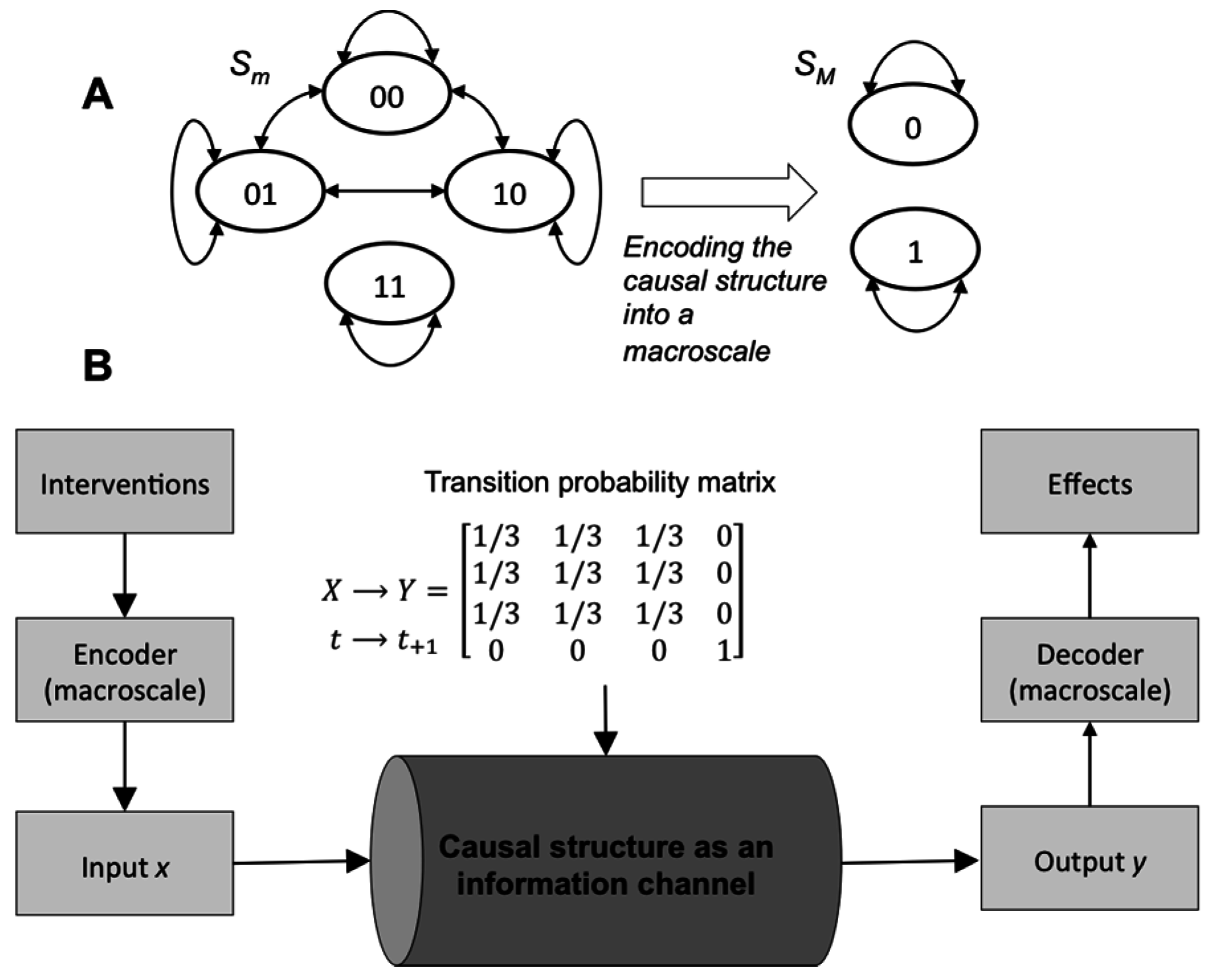
From this it is clear what higher spatiotemporal scales of a system are: a form of channel coding for causal structure. A macroscale is a code that removes the uncertainty of causal relationships, thus using more of the available causal capacity. An example of such causal coding is given using the TPM in Figure 2 with input X and output Y (t by t+1):
To send a message through a channel matrix with these properties one defines some encoding/decoding function. The message might be some binary string like {001011010011} generated via the application of some ID. The encoding function is a rule that associates some channel input with some output, along with some decoding function . The encoding/decoding functions together create the codebook. For simplicity issues like prefixes and instantaneous decoding are ignored here.
We can now define macro vs. microscale codes: an encoding function is a microscale code if it is a one-to-one mapping with a corresponding one-to-one decoding function: , as each microstate x is assumed to carry its own unique message. Intervening on the system in this way has entropy H(ID) = 2 bits as its four possible states are successive randomized interventions (so that p(1) = 0.5). Each code specifies a rate of transmission R = n/t, where t is every state-transition of the system and n is the number of bits sent per transition. For the microscale code of the system shown above the rate R = 2 bits, although these 2 bits are not sent reliably. This is because H(ID|ED) is large: 1.19 bits, so I(ID; ED) = H(ID) − H(ID|ED) = 0.81 bits. In application, this means that if one wanted to send the message {00,10,11,01,00,11}, this would take 6 interventions (channel usages) and there would be a very high probability of numerous errors. This is because the rate exceeds the capacity at the microscale.
In contrast, we can define a macroscale encoding function as the many-to-one mapping and similarly such that only macrostates are used as interventions (which is like assuming they are carrying a unique message). The rate of this code in the figure above is now twice as slow to send any message, as R = 1 bit, and the corresponding entropy H(ID) is halved (1 bit; so that p(1) = 0.83). However, I(ID; ED) = 1 bit, as H(ID|ED) = 0, showing that reliable interventions can proceed at the rate of 1 bit, higher than with using a microscale code. At the macroscales there would be zero errors in transmitting any intervention. This rate of reliable communication is equal to the capacity C.
Interestingly, it is therefore provable that causal emergence requires symmetry breaking. A channel is defined as symmetric when its rows p(y|x) and columns are permutations of each other. A channel is weakly symmetric if the row probabilities are permutations of each other and all the column sums are equal. For any such symmetric channel the input distribution that generates Imax has been proven to be the uniform distribution Hmax [22]. Treating the system at the microscale implies that ID = Hmax. Therefore, for symmetric or weakly symmetric systems, the microscale provides the best causal model without any need to search across model space. It is only in systems with asymmetrical causal relationships that causal emergence can occur.
6. Causal Capacity Can Approximate Channel Capacity as Model Choice Increases
The causal model that uses the full causal capacity of a system has an associated ID, which achieves its success in the same manner as the input distribution that uses the full channel capacity: by sending only a subset of the possible messages during channel usage. However, while the causal capacity is bounded by the channel capacity, it is not always identical to it. Because the warping of ID is a function of model choice, which is constrained in various ways (a subset of possible distributions), causal capacity is a special case of the more general channel capacity (defined over all possible distributions). Coarse-graining is one way to manipulate (warp) ID: by moving up to a macro scale. It is not the only way that the ID (and the associated ED) can be changed. Choices made in causal modeling a system, including the choice of scale to create the causal model, but also the choice of initial condition, and whether to classify variables as exogenous or endogenous to the causal model (“black boxing”), are all forms of model choice and can all also warp ID and change ED, leading to causal emergence.
For example, consider a system that is a Markov chain of 8 states:
where some states in the chain are completely random in their transitions. An ID of Hmax gives an EI of 0.63 bits. Yet every causal model implicitly classifies variables as endogenous or exogenous to the model. For instance, here, we can take only the last two states (s7, s8) as endogenous to the macro causal model, while leaving the rest of the states as exogenous. This restriction is still a macro model because it has a smaller state-space, and in this general sense also a macroscale. For this macro causal model of the system EI = 1 bit, meaning that causal emergence occurs, again because the ID is warped by model choice. This warping can itself be quantified as the loss of entropy in the intervention distribution, H(ID):
While leaving noisy or degenerate states exogenous to a causal model can lead to causal emergence, so can leaving certain elements exogenous.
Notably, there are multiple ways to leave elements exogenous (to not explicitly include them in the macro model). For instance, exogenous elements are often implicit background assumptions in causal models. Such background conditions may consist of setting an exogenous element to a particular state (freezing) for the causal analysis, or setting the system to an initial condition. Alternatively, one could allow an element to vary under the influence of the applied ID. This latter form has been called “black boxing”, where an element’s internal workings, or role in the system, cannot be examined [23,24]. In Figure 3, both types of model choices are shown in systems of deterministic interconnected logic gates. Each model choice leads to causal emergence.
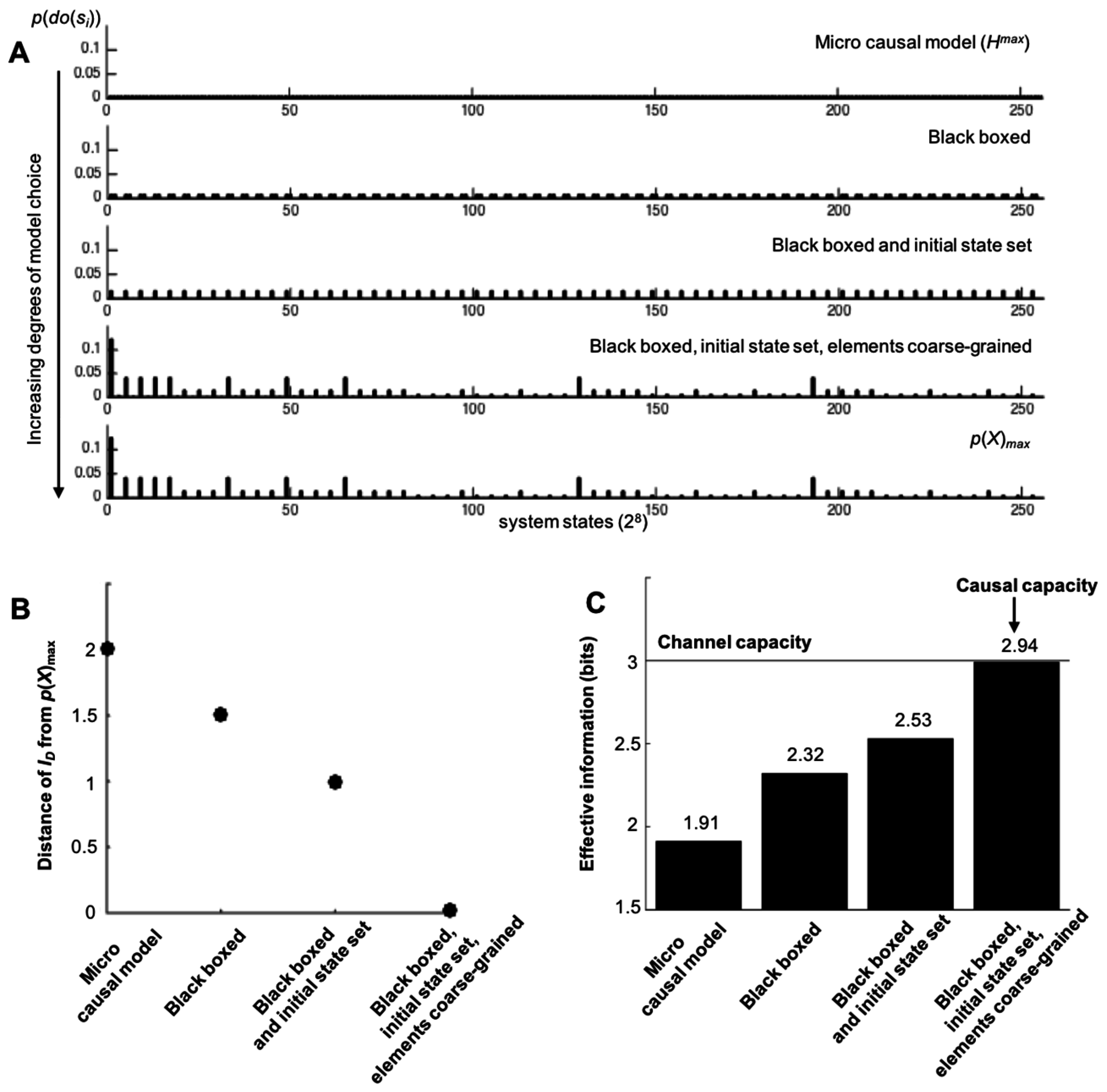
Rather than dictating precisely what types of model choices are “allowable” in the construction of causal models, a more general principle can be distinguished: the more ways to warp ID via model-building choices, the closer the causal capacity approximates the actual channel capacity. For example, consider the system in Figure 4A. In Figure 4B, a macroscale is shown that demonstrates causal emergence using various types of model choice (by coarse-graining, black-boxing an element, and setting a particular initial condition for an exogenous element). As can be seen in Figure 5, the more degrees of freedom in terms of model choice there are, the closer the causal capacity approximates the channel capacity. The channel capacity of this system was found via gradient ascent after the simulation of millions of random probability distributions p(X), searching for the one that maximizes I. Model choice warps the microscale ID in such a way that it moves closer to p(X), as shown in Figure 5B. As model choice increases, the EImax approaches the Imax of the channel capacity (Figure 5C).
7. Discussion
The theory of causal emergence directly challenges the reductionist assumption that the most informative causal model of any system is its microscale. Causal emergence reveals a contrasting and counterintuitive phenomenon: sometimes the map is better than the territory. As shown here, this has a precedent with Shannon’s discovery of the capacity of a communication channel, which was also thought of as counterintuitive at the time. Here an analogous idea of a causal capacity of a system has been developed using effective information. Effective information, an information-theoretic measure of causation, is assessed by the application of an intervention distribution. However, in the construction of causal models, particularly those representing higher scales, model choice warps the intervention distribution. This can lead to a greater usage of the system’s innate causal capacity than its microscale representation. In general, causal capacity can approach the channel capacity, particularly as degrees of model choice increase. The choice of a model’s scale, its elements and states, its background conditions, its initial conditions, what variables to leave exogenous and in what manner, and so on, all result in warping of the intervention distribution ID. All of these make the state-space of the system smaller, so can be classified as macroscales, yet all may possibly lead to causal emergence.
Previously, some have argued [26,27] that macroscales may enact top-down causation: that the higher-level laws of a system somehow constrain or cause in some unknown way the lower-law levels. Top-down causation has been considered as contextual effects, such as a wheel rolling downhill [28], or as higher scales fulfilling the different Aristotelian types of causation [29,30]. However, varying notions of causation, as well as a reliance on examples where the different scales of a system are left loosely defined, has led to much confusion between actual causal emergence (when higher scales are truly causally efficacious) and things like contextual effects, whole-part relations, or even mental causation, all of which are lumped together under “top-down causation.”
In comparison, the theory of causal emergence can rigorously prove that macroscales are error-correcting codes, and that many systems have a causal capacity that exceeds their microscale representations. Note that the theory of causal emergence does not contradict other theories of emergence, such as proposals that truly novel laws or properties may come into being at higher scales in systems [31]. It does, however, indicate that for some systems only modeling at a macroscale uses the full causal capacity of the system; it is this way that higher scales can have causal influence above and beyond the microscale. Notably, emergence in general has proven difficult to conceptualize because it appears to be getting something for nothing. Yet the same thing was originally said when Claude Shannon debuted the noisy-channel coding theorem: that being able to send reliable amounts of information over noisy channels was like getting something for nothing [32]. Thus, the view developed herein of emergence as a form of coding would explain why, at least conceptually, emergence really is like getting something for nothing.
One objection to causal emergence is that, since it requires asymmetry, it is trivially impossible if the microscale of a system happens to be composed only of causal relationships in the form of logical biconditionals (for which effectiveness = 1, as determinism = 1 and degeneracy = 0). This is a stringent condition, and whether or not this is true for physical systems I take as an open question, as deriving causal structure from physics is an unfinished research program [33], as is physics itself. Additionally, even if it is true it is only for completely isolated systems; all systems in the world, if they are open, are exposed to noise from the outside world. Therefore, even if it were true that the microscale of physics has this stringent biconditional causal property for all systems, the theory of causal emergence would still show us how to pick scales of interest in systems where the microscale is unknown, difficult to model, the system is open to the environment, or subject to noise at the lowest level we can experimentally observe or intervene upon.
Another possible objection to causal emergence is that it is not natural but rather enforced upon a system via an experimenter’s application of an intervention distribution, that is, from using macro-interventions. For formalization purposes, it is the experimenter who is the source of the intervention distribution, which reveals a causal structure that already exists. Additionally, nature itself may intervene upon a system with statistical regularities, just like an intervention distribution. Some of these naturally occurring input distributions may have a viable interpretation as a macroscale causal model (such as being equal to Hmax at some particular macroscale). In this sense, some systems may function over their inputs and outputs at a microscale or macroscale, depending on their own causal capacity and the probability distribution of some natural source of driving input.
The application of the theory of causal emergence to neuroscience may help solve longstanding problems in neuroscience involving scale, such as the debate over whether brain circuitry functions at the scale of neural ensembles or individual neurons [34,35]. It has also been proposed that the brain integrates information at a higher level [36] and it was proven that integrated information can indeed peak at a macroscale [16]. An experimental way to resolve these debates is to systematically measure EI in ever-larger groups of neurons, eventually arriving at or approximating the cortical scale with EImax [3,37]. If there are such privileged scales in a system then intervention and experimentation should focus on those scales.
Finally, the phenomenon of causal emergence provides a general explanation as to why science and engineering take diverse spatiotemporal scales of analysis, regularly consider systems as isolated from other systems, and only consider a small repertoire of physical states in particular initial conditions. It is because scientists and engineers implicitly search for causal models that use a significant portion of a system’s causal capacity, rather than just building the most detailed microscopic causal model possible.
Acknowledgments
Thanks to YHouse, Inc. for their support of the research and for covering the costs to publish. Thanks to Giulio Tononi, Larissa Albantakis, and William Marshall for their support during my PhD.
Conflicts of Interest
The author declares no conflict of interest.
References
- Fodor, J.A. Special sciences (or: The disunity of science as a working hypothesis). Synthese 1974, 28, 97–115. [Google Scholar] [CrossRef]
- Kim, J. Mind in a Physical World: An Essay on the Mind-Body Problem and Mental Causation; MIT Press: Cambridge, MA, USA, 2000. [Google Scholar]
- Hoel, E.P.; Albantakis, L.; Tononi, G. Quantifying causal emergence shows that macro can beat micro. Proc. Natl. Acad. Sci. USA 2013, 110, 19790–19795. [Google Scholar] [CrossRef] [PubMed]
- Shannon, C.E. A mathematical theory of communication. Bell Syst. Tech. J. 1948, 27, 623–666. [Google Scholar] [CrossRef]
- Granger, C.W.J. Investigating causal relations by econometric models and cross-spectral methods. Econometrica 1969, 37, 424–438. [Google Scholar] [CrossRef]
- Massey, J.L. Causality, feedback and directed information. In Proceedings of the International Symposium on Information Theory and Its Applications, Waikiki, HI, USA, 27–30 November 1990; pp. 303–305. [Google Scholar]
- Schreiber, T. Measuring information transfer. Phys. Rev. Lett. 2000, 85, 461–464. [Google Scholar] [CrossRef] [PubMed]
- Janzing, D.; Balduzzi, D.; Grosse-Wentrup, M.; Schölkopf, B. Quantifying causal influences. Ann. Stat. 2013, 41, 2324–2358. [Google Scholar] [CrossRef]
- Pearl, J. Causality; Cambridge University Press: New York, NY, USA, 2000. [Google Scholar]
- Tononi, G.; Sporns, O. Measuring information integration. BMC Neurosci. 2003, 4, 31. [Google Scholar] [CrossRef] [PubMed]
- Hope, L.R.; Korb, K.B. An information-theoretic causal power theory. In Australasian Joint Conference on Artificial Intelligence; Springer: Berlin/Heidelberg, Germany, 2005; pp. 805–811. [Google Scholar]
- Ay, N.; Polani, D. Information flows in causal networks. Adv. Complex Syst. 2008, 11, 17–41. [Google Scholar] [CrossRef]
- Griffith, P.E.; Pocheville, A.; Calcott, B.; Stotz, K.; Kim, H.; Knight, R. Measuring causal specificity. Philos. Sci. 2015, 82, 529–555. [Google Scholar] [CrossRef]
- Fisher, R.A. The Design of Experiments; Oliver and Boyd: Edinburgh, UK, 1935. [Google Scholar]
- Kullback, S. Information Theory and Statistics; Dover Publications Inc.: Mineola, NY, USA, 1997. [Google Scholar]
- Hoel, E.P. Can the macro beat the micro? Integrated information across spatiotemporal scales. Neurosci. Conscious. 2016, 2016, niw012. [Google Scholar] [CrossRef]
- Davidson, D. Essays on Actions and Events: Philosophical Essays; Oxford University Press on Demand: Oxford, UK, 2001; Volume 1. [Google Scholar]
- Stalnaker, R. Varieties of supervenience. Philos. Perspect. 1996, 10, 221–241. [Google Scholar] [CrossRef]
- Crutchfield, J.P. The calculi of emergence: Computation, dynamics and induction. Phys. D Nonlinear Phenom. 1994, 75, 11–54. [Google Scholar] [CrossRef]
- Shalizi, C.R.; Moore, C. What Is a Macrostate? Subjective Observations and Objective Dynamics. arXiv, 2003; arXiv:cond-mat/0303625. [Google Scholar]
- Wolpert, D.H.; Grochow, J.A.; Libby, E.; DeDeo, S. Optimal High-Level Descriptions of Dynamical Systems. arXiv, 2014; arXiv:1409.7403. [Google Scholar]
- Cover, T.M.; Thomas, J.A. Elements of Information Theory; John Wiley & Sons: Hoboken, NJ, USA, 2012. [Google Scholar]
- Ashby, W.R. An Introduction to Cybernetics; Chapman & Hail: London, UK, 1956. [Google Scholar]
- Bunge, M. A general black box theory. Philos. Sci. 1963, 30, 346–358. [Google Scholar] [CrossRef]
- Rubner, Y.; Tomasi, C.; Guibas, L.J. The earth mover’s distance as a metric for image retrieval. Int. J. Comput. Vis. 2000, 40, 99–121. [Google Scholar] [CrossRef]
- Campbell, D.T. ‘Downward causation’ in hierarchically organised biological systems. In Studies in the Philosophy of Biology; Macmillan Education: London, UK, 1974; pp. 179–186. [Google Scholar]
- Ellis, G. How can Physics Underlie the Mind; Springer: Berlin/Heidelberg, Germany; New York, NY, USA, 2016. [Google Scholar]
- Sperry, R.W. A modified concept of consciousness. Psychol. Rev. 1969, 76, 532. [Google Scholar] [CrossRef] [PubMed]
- Auletta, G.; Ellis, G.F.R.; Jaeger, L. Top-down causation by information control: From a philosophical problem to a scientific research programme. J. R. Soc. Interface 2008, 5, 1159–1172. [Google Scholar] [CrossRef] [PubMed]
- Ellis, G. Recognising top-down causation. In Questioning the Foundations of Physics; Springer International Publishing: Basel, Switzerland, 2015; pp. 17–44. [Google Scholar]
- Broad, C.D. The Mind and Its Place in Nature; Routledge: New York, NY, USA, 2014. [Google Scholar]
- Stone, J.V. Information Theory: A Tutorial Introduction; Sebtel Press: Sheffield, UK, 2015. [Google Scholar]
- Frisch, M. Causal Reasoning in Physics; Cambridge University Press: New York, NY, USA, 2014. [Google Scholar]
- Buxhoeveden, D.P.; Casanova, M.F. The minicolumn hypothesis in neuroscience. Brain 2002, 125, 935–951. [Google Scholar] [CrossRef] [PubMed]
- Yuste, R. From the neuron doctrine to neural networks. Nat. Rev. Neurosci. 2015, 16, 487–497. [Google Scholar] [CrossRef] [PubMed]
- Tononi, G. Consciousness as integrated information: A provisional manifesto. Biol. Bull. 2008, 215, 216–242. [Google Scholar] [CrossRef] [PubMed]
- Tononi, G.; Boly, M.; Massimini, M.; Koch, C. Integrated information theory: From consciousness to its physical substrate. Nat. Rev. Neurosci. 2016, 17, 450–461. [Google Scholar] [CrossRef] [PubMed]
Figure 1.
Markov chains with different levels of effectiveness. At the top are three Markov chains of differing levels of effectiveness, with the transition probabilities shown. This is assessed by the application of an ID of Hmax to each Markov chain, the results of which are shown as the TPMs below (probabilities in grayscale). The effectiveness of each chain is shown at the bottom.

Figure 2.
Causal models as information channels. (A) A Markov chain at the microscale with four states can be encoded into a macroscale chain with two states. (B) Causal structure transforms interventions into effects. A macro causal model is a form of encoding for the interventions (inputs) and effects (outputs) that can use a greater amount of the capacity of the channel. TPM probabilities in gray scale.

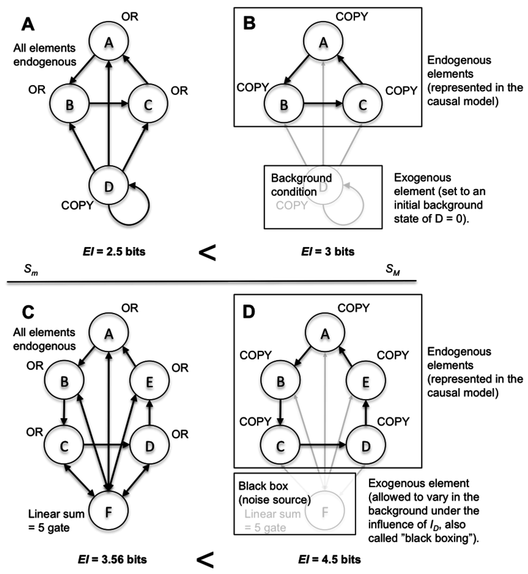
Figure 3.
Multiple types of model choice can lead to causal emergence. (A) The full microscale model of the system, where all elements are endogenous. (B) The same system but modeled at a macroscale where only elements {ABC} are endogenous, while {D} is exogenous; it was set to an initial state of 0 as a background condition of the causal analysis. (C) The full microscale model of a system with six elements. (D) The same system as in (C) but at a macroscale with the element {F} exogenous: it varies in the background in response to the application of the ID. EI is higher for both macro causal models.

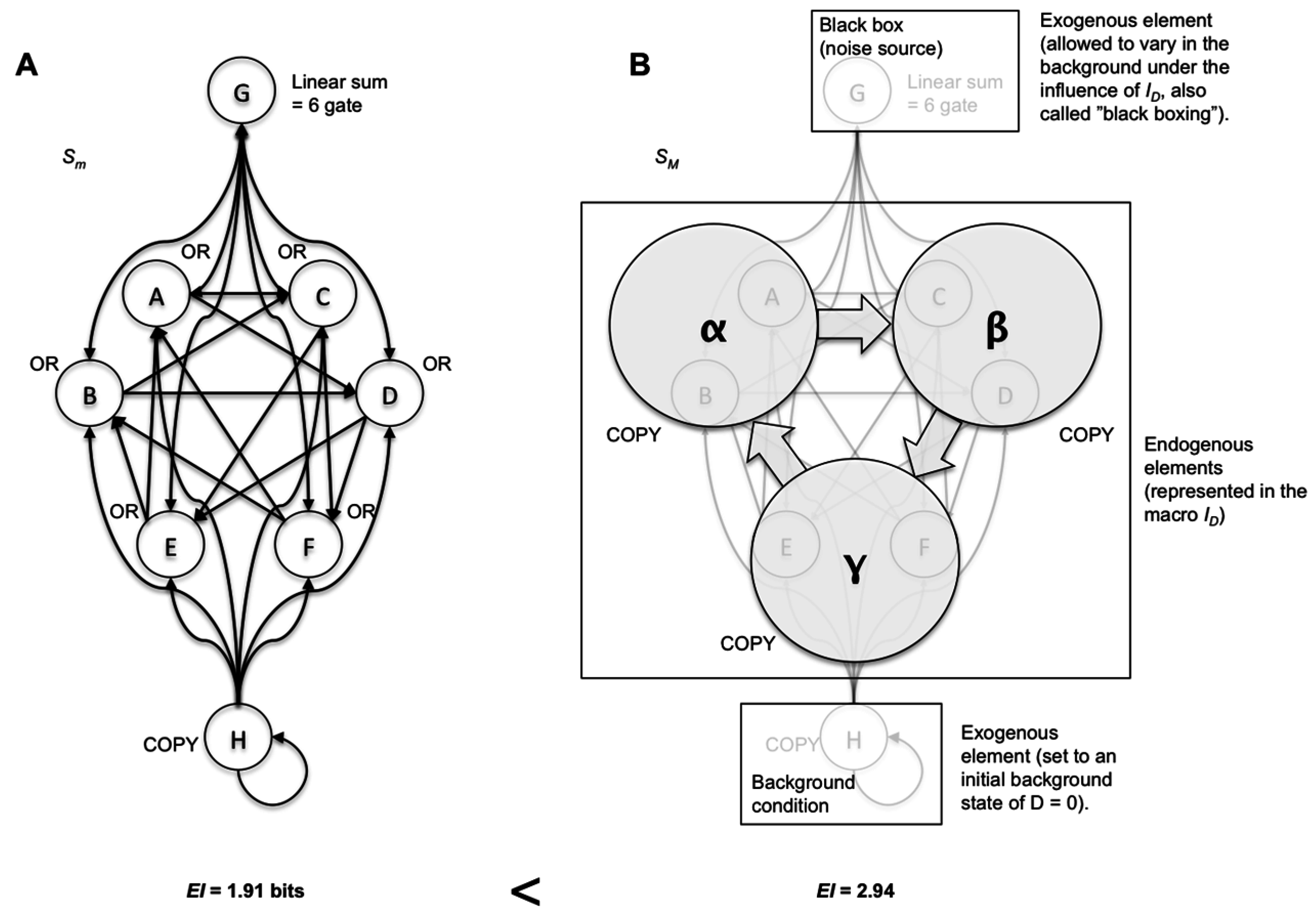
Figure 4.
Multiple types of model choice in combination leads to greater causal emergence. (A) The microscale of an eight-element system. (B) The same system but with some elements coarse-grained, others “black boxed”, and some frozen in a particular initial condition.
Figure 4.
Multiple types of model choice in combination leads to greater causal emergence. (A) The microscale of an eight-element system. (B) The same system but with some elements coarse-grained, others “black boxed”, and some frozen in a particular initial condition.

Figure 5.
Causal capacity approximates the channel capacity as more degrees of freedom in model choices are allowed. (A) The various IDs for the system in Figure 4, each getting closer to the p(X) that gives Imax. (B) The Earth Mover’s Distance [25] from each ID to the input distribution p(X) that gives the channel capacity Imax. Increasing degrees of model choice leads to ID approximating the maximally informative p(X). (C) Increasing degrees of model choice leads to a causal model where the EImax approximates Imax (the macroscale shown in Figure 4B).

© 2017 by the author. Licensee MDPI, Basel, Switzerland. This article is an open access article distributed under the terms and conditions of the Creative Commons Attribution (CC BY) license (http://creativecommons.org/licenses/by/4.0/).
Share and Cite
MDPI and ACS Style
Hoel, E.P. When the Map Is Better Than the Territory. Entropy 2017, 19, 188. https://doi.org/10.3390/e19050188
AMA Style
Hoel EP. When the Map Is Better Than the Territory. Entropy. 2017; 19(5):188. https://doi.org/10.3390/e19050188
Chicago/Turabian StyleHoel, Erik P. 2017. "When the Map Is Better Than the Territory" Entropy 19, no. 5: 188. https://doi.org/10.3390/e19050188
Note that from the first issue of 2016, this journal uses article numbers instead of page numbers. See further details here.