Article

An Explainable Artificial Intelligence Approach for Multi-Criteria ABC Item Classification

by
Alaa Asim Qaffas
1,*,
Mohamed-Aymen Ben HajKacem
2,
Chiheb-Eddine Ben Ncir
1,* and
Olfa Nasraoui
3
1
MIS Department, College of Business, University of Jeddah, Jeddah 23218, Saudi Arabia
2
LARODEC Lab, ISG Tunis, University of Tunis, Le Bardo 2000, Tunisia
3
Knowledge Discovery & Web Mining Lab, University of Louisville, Louisville, KY 40292, USA
*
Authors to whom correspondence should be addressed.
J. Theor. Appl. Electron. Commer. Res. 2023, 18(2), 848-866; https://doi.org/10.3390/jtaer18020044
Submission received: 19 January 2023 / Revised: 9 March 2023 / Accepted: 13 March 2023 / Published: 11 April 2023

Abstract

:
Multi-criteria ABC classification is a useful model for automatic inventory management and optimization. This model enables a rapid classification of inventory items into three groups, having varying managerial levels. Several methods, based on different criteria and principles, were proposed to build the ABC classes. However, existing ABC classification methods operate as black-box AI processes that only provide assignments of the items to the different ABC classes without providing further managerial explanations. The multi-criteria nature of the inventory classification problem makes the utilization and the interpretation of item classes difficult, without further information. Decision makers usually need additional information regarding important characteristics that were crucial in determining the managerial classes of the items because such information can help managers better understand the inventory groups and make inventory management decisions more transparent. To address this issue, we propose a two-phased explainable approach based on eXplainable Artificial Intelligence (XAI) capabilities. The proposed approach provides both local and global explanations of the built ABC classes at the item and class levels, respectively. Application of the proposed approach in inventory classification of a firm, specialized in retail sales, demonstrated its effectiveness in generating accurate and interpretable ABC classes. Assignments of the items to the different ABC classes were well-explained based on the item’s criteria. The results in this particular application have shown a significant impact of the sales, profit, and customer priority as criteria that had an impact on determining the item classes.

1. Introduction

Efficient inventory management plays an essential role in the management optimization of the overall supply chain. The procurement of raw materials and the manufacturing of products with the lowest stock-levels significantly contribute to cost reduction. Given that hundreds to thousands of items must be monitored and managed, it would be unrealistic to focus on each item separately. To address this issue, managers often attempt to use machine learning and data-driven methods to automatically classify items, commodities, and products into inventory classes in order to effectively manage each inventory group of items. This automatic process is referred to as inventory classification or item classification.
To effectively control the inventory and optimize the management of the supply chain, accurate inventory classification is required. Several methods and techniques for performing automatic inventory classification have been proposed [1,2,3]. ABC classification is one of the well used methods which divides inventory items into three managerial classes based on item description criteria. The first class, referred to as class A, contains a relatively small number of items that mostly contribute to the activity of the company. The second class, referred to as class B, includes items that are considered important, but having lesser importance than those of class A. The third class, referred to as class C, contains a large number of items having the least importance.
Although the classification of items was previously carried out based on one criterion, the “annual dollar usage” [4], several more recent works [5] in the literature consider other criteria as a basis for the classification of the items, including inventory holding unit cost, variability of replenishment lead time, scarcity, dependence to other items, substitutability, etc. The multi-criteria nature of the inventory classification problem makes the utilization and the interpretation of items classes, when these are derived from a black box process, difficult to understand. This is because knowing only which item belongs to which class is insufficient in real life business applications. Managers need to also understand which criterion and/or criteria has really contributed to the decision of assigning an item to a specific class rather than assigning it to the other classes. Unfortunately, when the automatic classification process operates as a black-box, it only gives a final organization of the items into three managerial classes without providing explanations about the reasons for assigning the items to a class. Yet, such explanations, when available, may help decision makers to transparently and effectively determine the right inventory management strategies for the items.
To solve this issue, we propose an eXplainable Artificial Intelligence (XAI) approach for multi-criteria ABC item classification. The proposed approach is based on the explainable artificial intelligence framework, SHape Additive exPplanations (SHAP), that provides an easy schematizing of the contribution of each criterion when building the inventory classes. It also allows to explain reasons behind the assignment of each item to any class. Such explanations make the resulting ABC inventory classes more transparent for decision makers. The rest of the paper is organized as follows: Section 1 gives an overview of inventory classification methods while describing the different criteria used to organize the inventory. Then, Section 2 describes the theoretical background for explainable artificial intelligence and the SHAP framework. Section 3 and Section 4 then describe the theoretical framework and empirical experiments for the proposed explainable clustering method for inventory organization. Finally, Section 5 gives the conclusion and future directions.

1.1. Literature Review of Inventory Classification Methods

Given the complexity of enterprise operations and architectures, an effective management of the inventory requires intelligent tools, techniques and methods to better increase service efficiency. In this context, ABC inventory classification is widely used to automatically organize the items into three groups of different managerial-levels and sizes. Several methods, based on different criteria and principles, have been proposed for ABC inventory classification [6,7,8]. Existing methods can be classified based on the used approach to building the different classes. These approaches can be categorized into: (i) Decision making, (ii) Mathematical programming and (iii) Machine learning and soft computing approaches. We review these approaches below.
The first category of item classification methods, decision-making methods, are based on probabilistic or conceptual data modeling techniques to look for an optimal classification of the items. Usually, these methods consist of several phases to solve the multi-criteria problem. An example of such methods is the Analytic Network Process (ANP) method [9] for evaluating the logistic strategies and the production speed. This method models the multi-criteria problem by a network involving the internal dependency of criteria to make the decision-making more efficient. Other existing works [10,11] proposed to extend Annual Dollar Usage, and Scoring methods to build an ABC classification of the items. Examples of such methods are those proposed by Liu and Hung [10] who proposed a Data Envelopment Analysis (DEA) model to define the ABC classes and Onwubolu and Dube [11] who proposed using spreadsheets to solve the multi-criteria problem. More recent decision-making methods have been proposed to build inventory classes such as the works of Zheng et al. [12] who applied Shannon’s entropy to look for optimal ABC classes and the works of Wu et al. [13] who used the weighted least-squares dissimilarity approach to obtain a set of local item weights which are then aggregated in the overall evaluation score function. Another interesting decision-making system is proposed in the works of Eraslan and Ic [3] who developed an efficient decision support system to help decision-makers build the ABC classes of the items. This system gives high flexibility to decision-makers by introducing subjective criteria.
The second category of item classification methods, mathematical programming methods, are essentially based on linear and nonlinear programming models to build a vector or a matrix that optimizes weighted item scores. An overall score is usually calculated by an objective function that would be optimized. Examples of conventional mathematical programming methods include the weighted linear optimization model [14] and the Ng-model [15]. Extensions of the Ng-model were presented in the works of [16] that proposed both the H-model and F-model approaches. More recent mathematical-based methods incorporate a cross-efficiency evaluation method into a weighted linear optimization model for ranking the items, as presented in the works of [2] which proposed a Cross-Evaluation methodology to optimize the weighted linear optimization problem. In addition, the work in [17] integrated an alternative overall measure within the Ng-model to optimize the descending ordering of the items.
The third category of existing methods comes from the machine learning and soft computing domains. A learning process is integrated that allows estimating the final assignment of the items while optimizing a learning model or an objective function. Several machine learning classification methods are used to build the ABC classes such as k-means, Fuzzy c-means (FCM), K-nearest neighbors and Support Vector Machines (SVM) algorithms. In [18], Chu et al. proposed the ABC-Fuzzy Classification (ABC-FC) method which is based on the Fuzzy c-means (FCM) algorithm and incorporates decision makers’ judgment of inventory classification. In the same way, Keskin and Ozkan [1] and Cebi et al. [19] proposed to design an FCM-based process to solve the multi-criteria classification problem in order to help managers make better decisions under fuzzy circumstances. In the works of [5], the authors proposed the AHP–FCM–Rveto method that is based on three phases to build the final inventory classes which are AHP phase, FCM phase and Revised-Veto phase. Other machine learning techniques have been used to build the ABC classes such as Artificial Neural Networks. Partovi and Anandarajan [20] proposed a genetic algorithm (GA)-based learning method to develop an artificial neural network for inventory classification. The obtained results have shown that neural network-based inventory classification can give higher predictive accuracy than conventional inventory classification methods. An interesting comparative study is presented in the works of [21]. The authors compared the performance of three machine learning-based classification models, namely SVM, Back Propagation Networks and KNN when building inventory classes.

1.2. ABC Inventory Classification: Problem Definition and Challenges

Let X = x 1 x n be a dataset of n inventory items, also called Stock Keeping Units (SKU), where each item x i is described over m quantitative criteria j 1 , j 2 , . . . , j m . We also assume that the m criteria are of benefit-type and have a positive relation to the importance level of the items. If one criterion is not positively related to the importance level of the items, the reciprocal can be used to make it positively related. The objective of the ABC inventory classification process is to organize the n items into three groups (classes) of different sizes namely A, B and C. The distribution of the items over the three different groups must follow as follows: class A items will be a small percent of inventory, but contribute most in terms of activity and revenue, class C items will form a large percent of inventory, but contribute the least to activity and revenue, and finally, class B items will fall in the middle. Theoretically, ABC aims to build an assignment matrix U ( n , 3 ) where each row i corresponds to an item x i , and each column t represents one class. The matrix values u i t , i [ 1 . . n ] , t [ 1 . . . 3 ] are binary where the value u i t = 1 corresponds to the categorization of an item x i as belonging to the class t. To meet the ABC classification model principles, the sizes of class A, B and C must be in the intervals [ 10 % . . . 20 % ] , [ 20 % . . . 30 % ] and [ 50 % . . . 70 % ] , respectively. Figure 1 gives an overview of the inputs and outputs of the multi-criteria ABC inventory classification process.
In this work, we focus on learning-based multi-criteria ABC inventory classification methods which are usually based on the application of conventional clustering techniques to build the different ABC classes. Although this category of methods has been widely used and has shown good performance, it raises the issue of non-explainability and non-transparency of results in real-life applications. In fact, the clustering algorithm works like a black-box process that ends by giving a final categorization of the items into three groups without giving sufficient explanations relative to the decision of assigning an item to any particular class. In practice, given the multi-criteria nature of the problem, managers usually need additional information regarding the criterion (or criteria) that was crucial in determining the assignment of an item to the A, B or C class. Such information allows a better analysis of the items, allows easy detection of miss-classified items, helps managers to better understand the inventory groups and makes inventory management decisions more flexible. To the best of our knowledge, there is no existing work that studied the explainability of ABC inventory classes.
To deal with the non-explainability of ABC inventory classes, we propose a new multi-criteria ABC inventory classification approach based on Explainable Artificial Intelligence (XAI) capabilities. We present, in the next section, the background and basic concepts of the used approach.

2. Background on Explainable Clustering

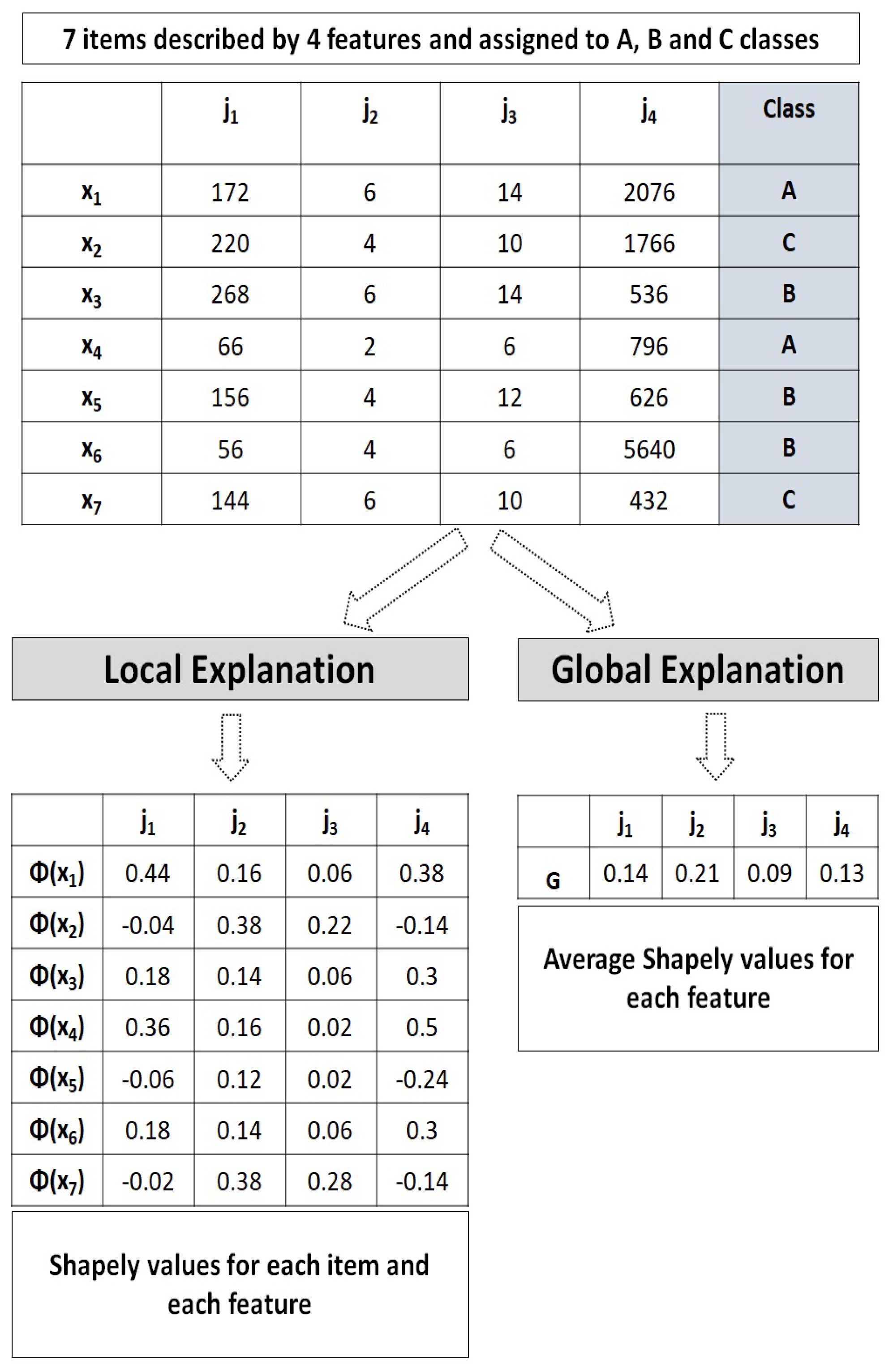
2.1. Explainable Clustering

Clustering offers a solution to analyze a large amount of real-world unlabeled data. However, most of the existing clustering methods do not provide a way for decision-makers to understand their results especially for non-domain experts. Hence, these methods act as “black-boxes” and build clusters without providing any explanations regarding the reasoning behind their creation. This issue reduces user trust and makes interpretations and choices less transparent.
Explainable clustering, a branch of Explainable Artificial Intelligence (XAI), attempts to address this problem by allowing decision-makers to interpret and evaluate the clusters by providing additional explanations of used features. XAI methods were firstly designed to interpret complex supervised methods by focusing on feature importance in black-box models [22]. Several XAI methods were proposed in the literature [22,23,24] which can be classified into model-specific and model-agnostic. Model-agnostic methods can be applied to any machine-learning model. Typically, model agnostic models require labels on data records to achieve interpretability. Model-specific methods are restricted to a particular model. Small decision trees are one such example of model specific interpretable model, as the splitting criteria used to explain decision trees are restricted to decision tree algorithms. All of these methods provide either Local or global explanations, or both at once. Local explainability can be used to explain why a specific data point belongs to a given class or how to change the label of a data point by changing its feature values. Global explainability can be defined as generating explanations on why a set of data points belongs to a specific class, the important features that decide the similarities between points within a class and the feature value differences between different classes.
In the same way as for supervised models, explainability was also studied for unsupervised models, especially clustering methods. Existing explainable clustering methods try to generate explanations in terms of the underlying features used in the black-box clustering process. Some existing explainable methods [25,26,27] were proposed, to visualize the resulting clusters across two or three Principal Component Analysis (PCA) axes. The main limitation of these methods is the dimensionality reduction, which does not show relationships between the clusters and the original features. Furthermore, cluster interpretations become difficult since PCA axes cannot be readily interpreted in the case of input features. Other existing explainable clustering methods propose to generate cluster representatives to facilitate the understanding of clusters by either computing cluster-centroids or by choosing a small subset of data objects [28,29,30]. These methods may make it easier to analyze each cluster through a simple interpretation of the cluster representatives, but they are particularly sensitive to the geometry of clusters and assume a strict feature similarity between data objects within a cluster, which is not the case in real life-applications.
Recently, a two-step process was proposed for explainable clustering [31,32,33] to explain the clusters using recent XAI agnostic-method. The first step is devoted to the label assignments (i.e., clusters), then in the second step, these labels are used as target variables in a classification task. Explanations are then built based on the obtained supervised learning model. For example, researchers in [33] have used existing supervised XAI methods for interpreting clustering approaches (EXPLAIN-IT). First, they cluster the input data using existing clustering methods such as K-Means or DBSCAN. A classifier is then trained on input data using the generated cluster labels as class labels for the classifier. Finally, the classifier is explained using existing model agnostic methods such as LIME [34]. LIME is one of the most popular interpretability methods, which can generate interpretations for a single prediction produced by any classifier. Although LIME is powerful and straightforward, it was designed for mainly providing local explanations. So, we propose in this paper to use the SHAP method to improve the explanations of the ABC item classification. SHAP can provide local and global explanations at the same time, and it has a solid theoretical foundation compared to other XAI methods [35].

2.2. SHAP (Shapley Additive Explanations)

SHAP is a model-agnostic XAI method, used to interpret predictions of machine learning models [36]. It is based on ideas from game theory and provides explanations by detecting how much each feature contributes to the accuracy of the predictions. SHAP also provides the most important features and their impact on model prediction. It uses the Shapley values to measure each feature’s impact on the machine learning prediction model. Shapley values are defined as the (weighted) average of marginal contributions. It is characterized by the impact of feature value on the prediction across all possible feature coalitions. The Shapley value for an instance x is defined as follows:
ϕ j r ( x ) = S { j 1 j m } { j r } η m ! × ω j r
with
ω j r = [ φ S j r ( x ) φ S ( x ) ]
η = ( m S 1 ) ! × S !
where ϕ j r ( x ) denotes the Shapley value for the feature value having the index j r [ 1 . . m ] , S is a subset of the features used in the prediction model, | S | is the cardinality of S, m denotes the number of features, φ S j r ( x ) and φ S ( x ) are the prediction function for the set of feature values in S with and without including the feature j r , respectively. The Shapley value ϕ j r ( x ) measures how much the feature j r contributes to the prediction model, either positively or negatively. For that reason, the model is trained with and without including this feature and then predictions from the two models are compared for all feature subset S { j 1 , . . . , j m } { j r } . When ϕ j r ( x ) is a large positive value, it means that feature j r has a large positive impact on the prediction model. However, when this value is negative, it means that feature j r has a large negative impact on the prediction model.

3. Proposed Explainable Clustering Method for Multi-Criteria ABC Inventory Classification

In order to deal with the complexity of explaining ABC inventory classes, we propose a new explainable clustering approach based on both k-means based clustering and XAI capabilities. The proposed approach, referred to as Explainable k-means (Ex-k-means), includes two main phases: item classification and explanation generation. In the first phase, a k-means-based clustering is applied to guide the item classification process to build three classes having varying sizes respecting the ABC distribution of the items. A second phase, the ABC-inventory-interpretation phase, is devoted to improving the transparency of the obtained ABC classes based on the XAI SHAP method capabilities. Because the transparency and the easy-interpretation of inventory classes are almost as important as item classification accuracy, SHAP-based process is designed to have as outputs detailed explanations of the global structure of inventory classes as well as local explanations of the assignment of each item to any specific ABC class. Figure 2 gives an overview of the two main phases of the proposed explainable clustering approach as well as the inputs and outputs of the proposed approach.

3.1. Phase 1: Item Classification

This phase uses, as inputs, the numerical description of the set of items and returns, as outputs, the built ABC inventory classes by using a k-means clustering process. This process aims to build three ABC inventory classes based on an alternating iterative process.
Given a dataset X = x 1 x n containing n items, described by m criteria, the aim of Ex-k-means is to find k = 3 clusters { U 1 A , U 2 B , U 3 C } by minimizing the overall within-cluster-sum-of-squares, denoted (J), as follows:
J = i = 1 n t = 1 k u i t d ( x i , r t ) ,
where u i t takes value 1 if item x i is assigned to cluster t or 0 otherwise, r t { r A , r B , r C } is the representative of cluster t and d ( x i , r t ) is the Euclidean distance between x i and cluster representative r t . The cluster Representative r t is calculated for each cluster t by:
r t = i = 1 r t x i r t ,
where r t the number of items assigned to cluster t.
The minimization of the overall within-cluster-sum-of-squares (J) is performed by using an alternating optimization of two independent sub-steps: item assignment and update of the set of clusters representatives { r A , r B , r C } . The first sub-step assigns each item to the nearest cluster representative. After assigning all items, the next sub-step updates the new cluster representative of each of the three ABC clusters. These two sub-steps are repeated until convergence is reached. The convergence is characterized by a maximal number of iterations or no improvement in the objective criterion between two repeated iterations.

3.2. Phase 2: ABC-Inventory-Interpretation Phase

The goal of this phase is to generate the explanations for the ABC classes which are obtained in the previous phase. These explanations help decision makers to understand and interpret the final ABC item classification in terms of local and global built structures. Local explanations have the objective to explain the reasons behind the assignment of each item to any ABC class in terms of feature values while global explanations try to explain important feature values for each ABC class. The proposed explanation phase is based on the SHAP method. First, the resulting ABC clusters are configured as the target supervised variables of the explainable process. Then, local and global explanations are built by using the SHAP functionalities.
For local explanations of the items, we compute the Shapley value at the item level for each criterion with respect to the assigned ABC class. These Shapley values objectively quantify the contribution of each criterion when deciding to assign any items to the ABC classes. These local explanations allow decision makers to understand the reasons behind assigning an item to the A, B or C class. The decision-makers can also evaluate the impacts of increasing or decreasing the criterion value of each item on the predicted class label.
For global explanations, we provide detailed explanations regarding the importance and contributions of the features when building each ABC class. Local Shapley values of data items are summarized and used as “atomic units” for building the global explanations as follows:
G j = 1 n i = 1 n ϕ j ( x i )
where ϕ j ( x i ) denotes the Shapley value of criterion j for item x i , G j refers to the overall Shapley value of criterion j and n is the total number of items in the dataset. Global Shapley values are then sorted in decreasing order to show the most important feature when building ABC classes.
We give, in the following, an illustrative example of local and global explanations. Let us consider a small dataset including 7 items that are described by 4 criteria j 1 , j 2 , j 3 , and j 4 , we want to interpret the multi-criteria ABC classification of these items in terms of the local and global explanations. Figure 3 illustrates the outputs of the proposed explanation process based on the SHAP method. First, the Shapley value of each data item and each criterion is calculated with respect to the class label using Equation (1). Then, an average of Shapley values from each criterion are summarized using Equation (6).
For local explanations, criteria with high Shapley values are interpreted as having high impact on the decision of item assignments, whereas criteria with low Shapley values have lower impact. In fact, it is important to note that criteria with high Shapley values are interpreted as pushing toward one class and low Shapley values as pushing towards the other classes. For example, for item x 4 , we can see that the criteria with the highest Shapley values are j 1 and j 4 while for the item x 2 , criteria with the highest Shapley values are j 2 and j 3 . For global explanations, the criteria with the highest values are interpreted as largely contributing to the decision of class labels of the items. For example, we can observe that the first criterion ( j 2 ) has the largest contribution in the decision of building the overall ABC classes while the third criterion ( j 3 ) has the lowest contribution.

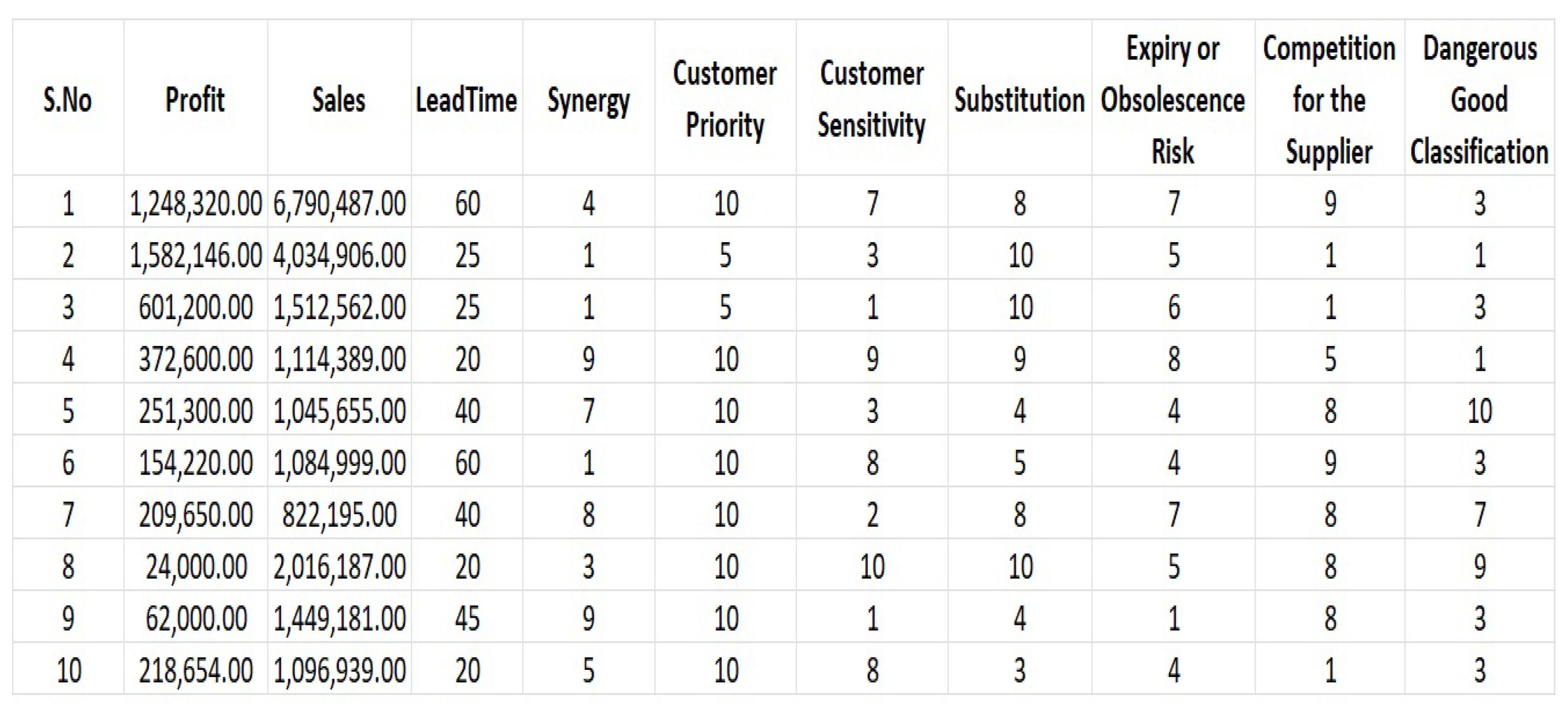
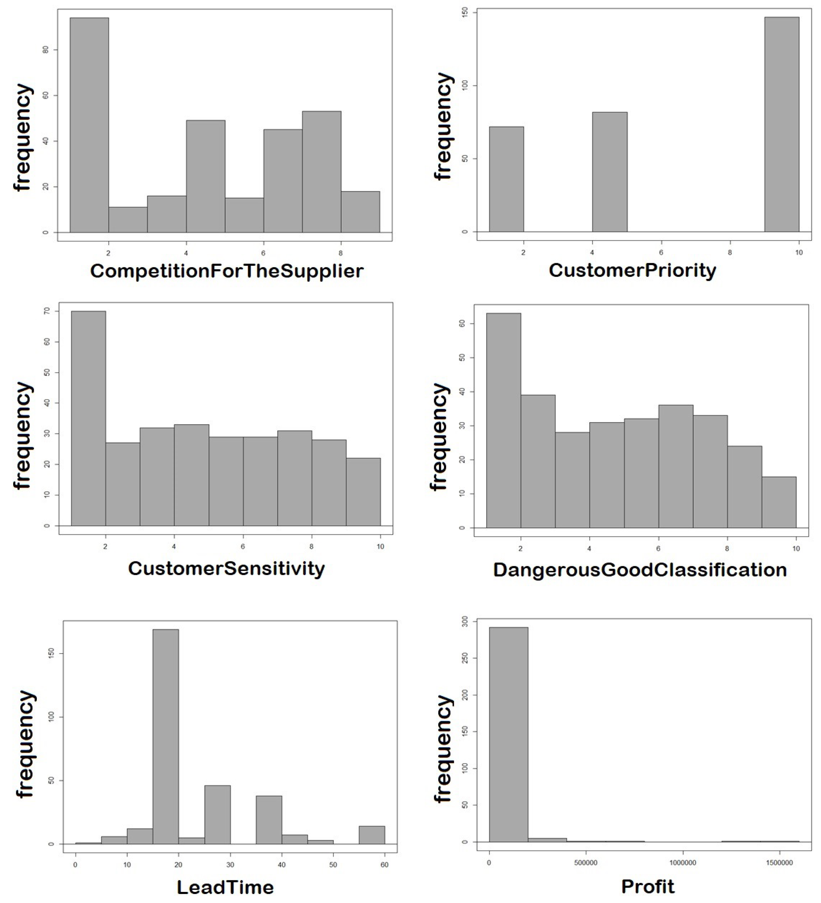
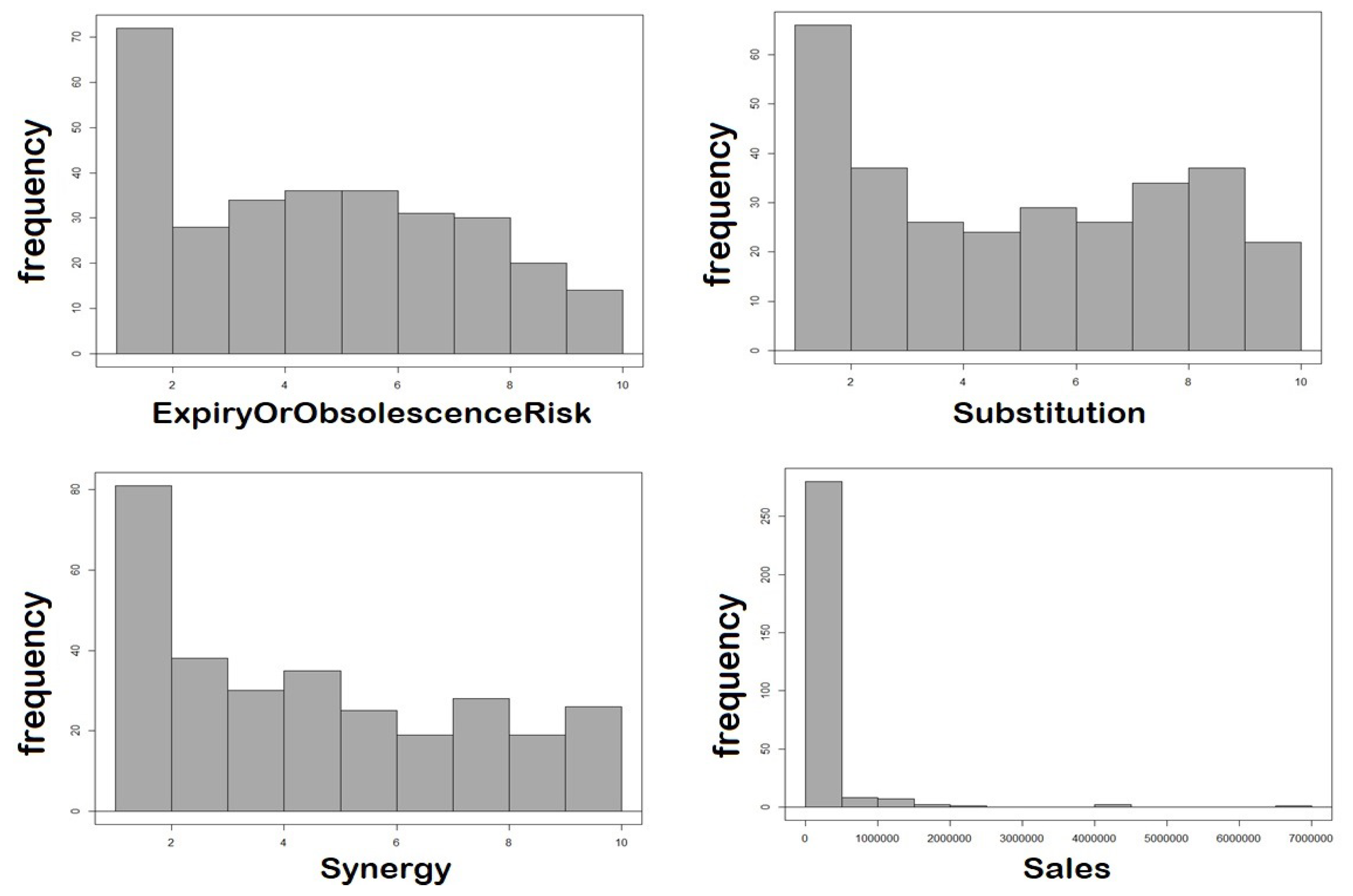
4. Experiments and Results

We use a dataset from a company specializing in retail sales. An extract of the first tenth raw data is reported in Figure 4. The dataset contains 301 inventory items described by 10 numerical criteria as follows: Sales, Profit, Lead time, Synergy, Customer priority, Customer sensitivity, Substitution, Expiry or obsolescence risk, Competition for the supplier, Dangerous good classification. Figure 5 reports histograms of data values and their respective frequencies for each criterion. A multi-criteria ABC inventory classification seems mandatory for the company to help decision-makers automatically define different managerial levels for the set of items.
We begin by studying the data variability for all the item criteria. Table 1 shows minimum, 1st quartile, median, mean, 3rd quartile and maximum values for each criterion. This table shows good data centrality around the median and mean except for those obtained for Profit, Sales and Lead Time. These three criteria also have large scales compared to the other criteria, which require normalized data before building the ABC clusters. A min-max normalization [ 0 . . . 1 ] was performed using the following formula:
x ˇ i j = x i j x j m i n x j m a x x j m i n
where x ˇ i j is the normalized value of the data item x i for criterion j, x j min is the minimum value of criterion j and x j max is the maximum value of criterion j. Once data are normalized, we used the proposed Ex-k-means algorithm, to build the different ABC classes.

4.1. Evaluation of the Clustering Performance

We evaluate the performance of the proposed explainable clustering method compared to existing ones AHP-k-means [37], AHP-k-means-Veto [37], AHP-FCM [5] and AHP-FCM-Rveto [5]. Table 2 shows the cluster-sizes obtained by each method by fixing the number of clusters k = 3 for all methods. We assigned the A, B and C classes respecting the sizes of the built clusters from lowest to highest, respectively, (class A for the cluster with the minimal size). Table 2 shows that AHP–FCM, AHP–FCM–Rveto and Ex-k-means methods gives a good distribution of the items over the three classes. We show large differences in the sizes of the obtained ABC classes. AHP-k-means and AHP-k-means-Veto build a cluster (Class A items) with very small size. The AHP-FCM-Rveto method build the best distributed clusters, based on the ABC principles, given its integrated Rveto phase.
Next, we evaluate the quality of the obtained ABC clusters by using the internal validation measures, Silhouette Coefficient (SC) [38], Davies–Bouldin Index (DBI) [39], and Calinski–Harabasz Index (CHI) [40]. These validation measures aim to measure the compactness and separation of the clusters. Compactness measures how closely related the items in a cluster are while separation measures how distinct or well-separated a cluster is from other clusters. Higher values of the SC and DBI measures indicate a good quality partition, while lower values of the CHI measure indicate the best partition. The results are reported in Table 3. This table shows that the proposed Ex-k-means method outperforms the compared methods in terms of DBI and CHI measures.

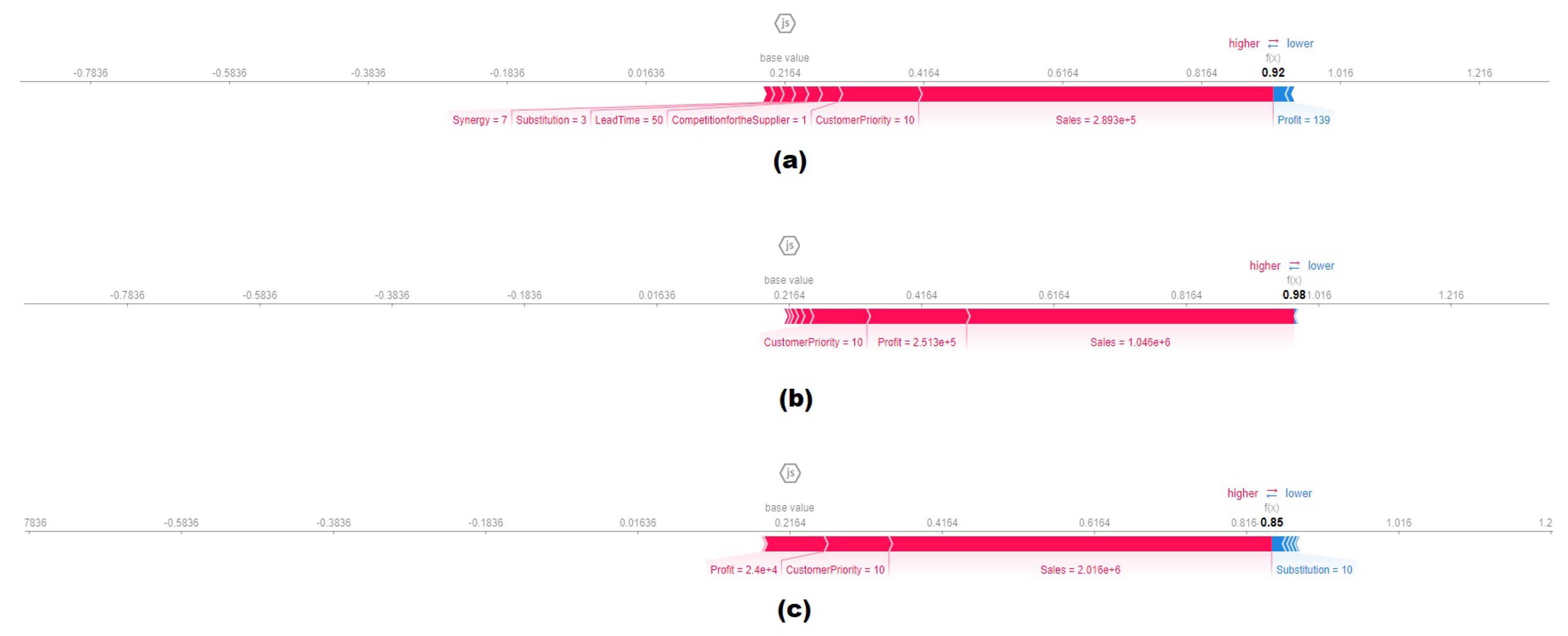
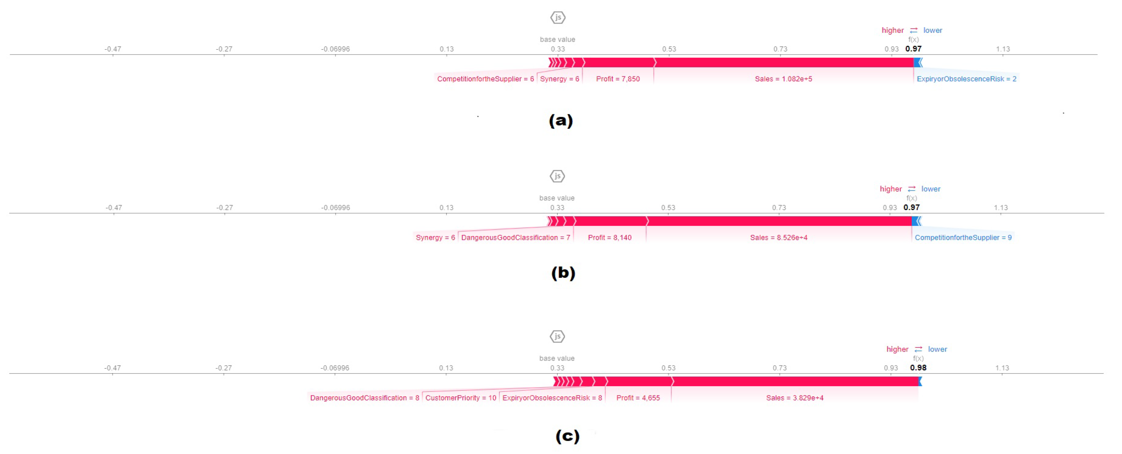
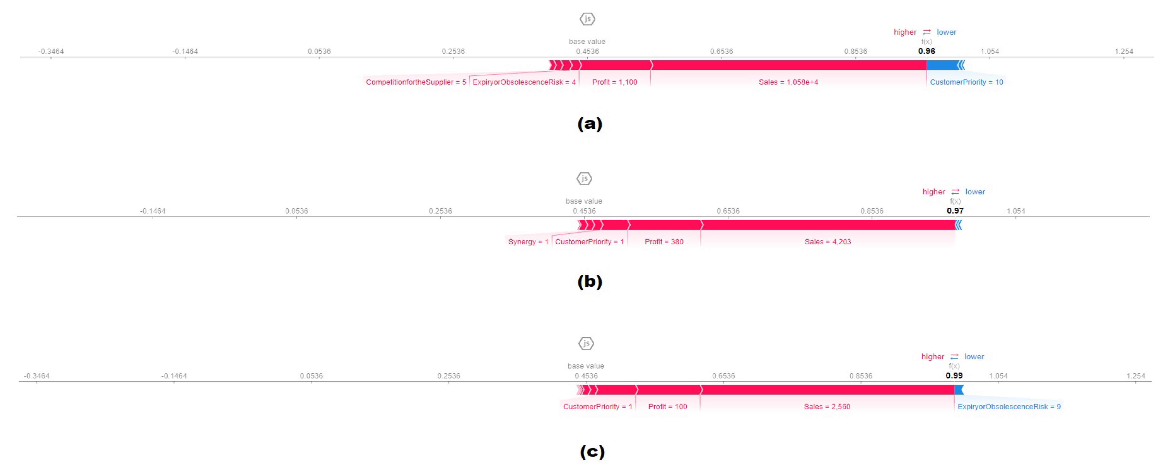
4.2. Local Explanations of Item Assignment to the ABC Classes

The local explanation has the objective to build an easy item-interpretable model explaining the decision behind the assignment of each item to any ABC class. We used the force plot which schematizes how features contributed to the cluster assignment of each item separately. This plot provides a deep understanding and easy interpretation of the classification of any particular item. We randomly selected a set of 3 items from each class and then the force plot of Shapley values of each item is reported. Figure 6, Figure 7 and Figure 8 show the contribution of each criterion, at the item level, when building the ABC inventory classes. The bold numeric values on the right side of these figures evaluate the probability of the decision of assigning one item to its current class rather than any other class. We obtain a high probability for the selected items from all classes (higher than 97 % ) except for the probability reported for the third item assigned to class A (Figure 6c) which reports a probability of 85 % . High probability indicates the facility of identifying the respective class of the item by using the proposed classification model. However, any item with a low probability value, or a probability converging to the base value, indicates the difficulty of determining its correct class given its dissimilarity with all built classes. The base value is the average value that would be predicted if we did not know any criteria for the current item. The base value is the average of the model labels in the training dataset. We show in Figure 6, Figure 7 and Figure 8 that base values correspond to the considered cluster-sizes ( 20 % , 30 % and 50 % ) for the A, B and C classes, respectively.
The reported numbers below the plot arrow represent the value of each criterion for that item. Two colors are then used to schematize criteria value impact: red for criteria values that pushed the model classification probability higher and blue for criteria values that pushed the model classification probability lower. The bigger the arrow size, the bigger the impact of the criterion on the model classification. Figure 6 shows that the decision of assigning the selected set of items to class A was based on a very high value of sales (average ≃1,100,000 for the three selected items), high Profit (average ≃92,000 for the three selected items) and high Customer priority (≃10). All these criteria values have positively contributed (red color) to increase the probability of assigning the respective items to class A. Figure 6a,c show that the decision of assigning the respective items to class A has been negatively (blue color) affected by the low value of profit (≃139) for the first item and the high value of substitution (≃10) for the second item. This fact explains the low reported probabilities in Figure 6a,c compared to the reported probability in Figure 6b.
Concerning the items of class B, Figure 7 shows that the decision of assigning these items was based on moderate volumes of Sales (Average ≃77,000 for the three selected items), high profit Profit (average ≃7000 for the three selected items), high values of both Synergy (≃6) and CompetitionForTheSupplier (≃6). These criteria values increase the probability to judge the item as belonging to class B. All these criteria values lie between the average and the third quartile values. However, Figure 7a,b show that a low value of Expiry Obsolescence Risk (≃2) and a high value of Competition For The Supplier (≃9) slightly decrease (blue color) the probability of assigning these two items to class B.
Items of the third class, class C, are reported in Figure 8. This figure shows that criteria values which mostly contributed to the assignment of these items are very low Sales Volume (average ≃5700 for the three selected items), very low Profit (average ≃500 for the three selected items) and moderate values of both Expiry obsolescence risk (≃5) and Competition For the Supplier (≃5). All these low criteria values increase the probability of assigning the items to class C, while it is not the case for the high value of Customer priority (≃10) (reported in Figure 8a) that highly reduces the probability of assigning the respective item to class C.
These locally built explanations can be very useful to decision-makers for a deep understanding of the assignment of each item separately. In some cases, further analysis would be required to decide the class of some items, especially those having low classification probability. The local explanations increase the classification model transparency and improve the quality of determining the right managerial classes for the items.

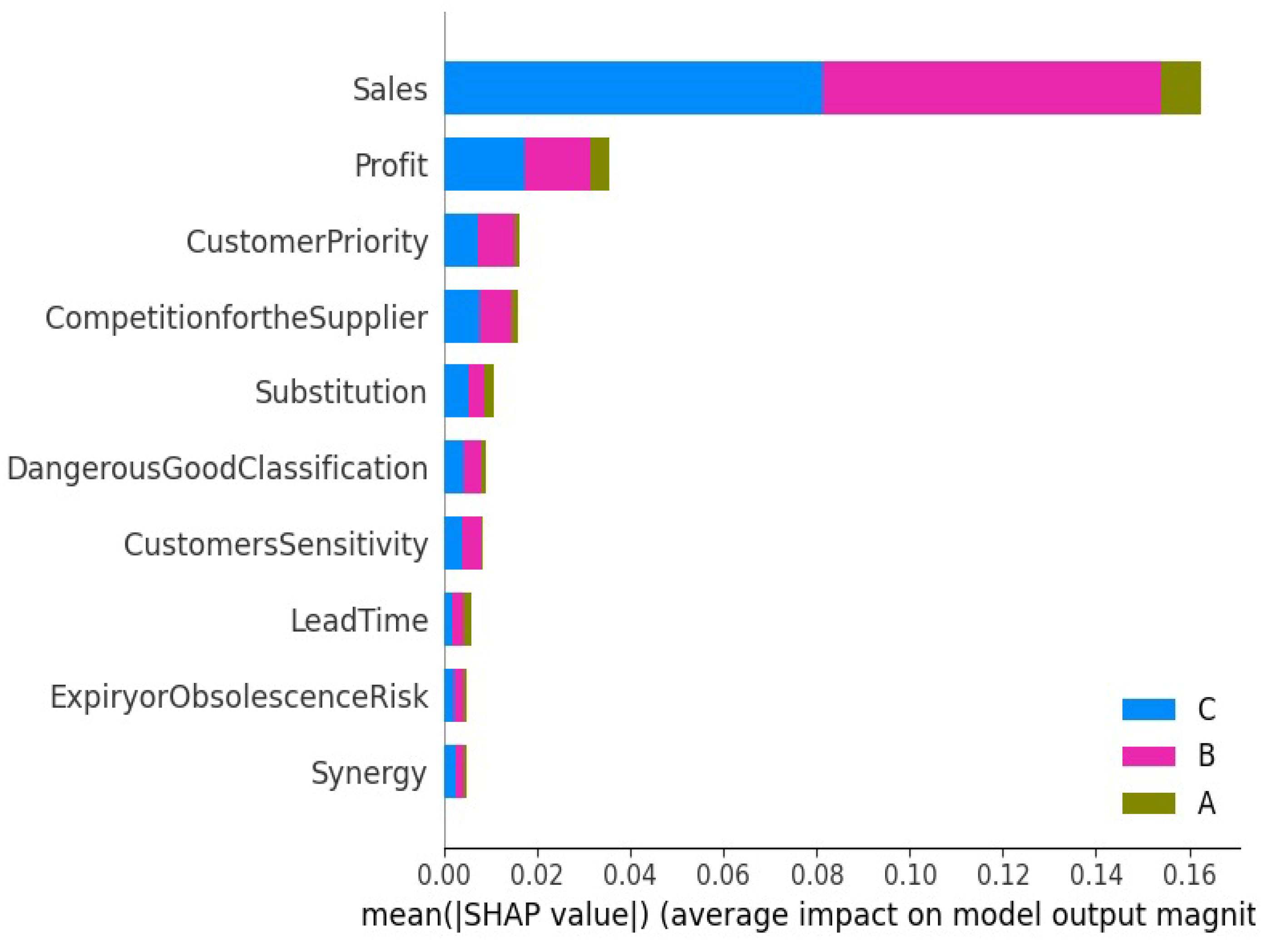
4.3. Global Explanations of ABC Classes

Global explanations have the objective of easily interpreting the ABC classification model at the level of classes rather than the local item level. For each ABC class, the criteria that mostly contributed to the decision of assigning items to a specific class are stacked and reported. We used the feature-importance plot, in which items Shapley values are summarized for each class separately. Figure 9 reports the most important criteria after summarizing shape values for items assigned to A, B and C classes separately. These criteria are schematized according to their contribution to the classification model from highest (at the top of the plot) to lowest (at the bottom of the plot). The contribution of each criterion within each class is reported with a different color: navy-green for class A, pink for class B and blue for class C. Figure 9 shows that Sales, Profit, Customer priority, and Competion for the supplier criteria have the largest impact on the classification model compared to the other criteria. In addition, we can see that the criterion Customer priority largely contributes to determining class B items compared to the other classes. We can also see that Expiry or obsolescence risk and Synergy criteria have the same low contribution for all classes. These findings are broadly in accordance with the literature on inventory classification.
The feature-importance plot only shows the importance of each criterion when building the ABC classes, without explaining its impact (positively or negatively) on the classification model. In order to show criteria impacts for each class, we build the feature-summary-plot that combines feature importance and impact. Figure 10 shows the positive and negative relationships of criteria values with the target class. Every single point in these sub-figures is a Shapley value of one criterion for a specific item. The position on the y-axis is determined by the criterion, and the x-axis is determined by the Shapley value. The color represents the criterion value from low (blue) to high (red). First, this figure confirms the finding that Sales and Profit criteria have the highest importance when deciding the inventory class of any item and for the three classes A, B, and C. On the other hand, Lead Time, Expiry obsolescence risk and Synergy have the lowest importance which tends to be negligible. Besides, Figure 10a shows that the larger the values of Sales and Profit (red points), the larger the Shapley value is (points are located at the right of the x-axis). This shows the positive impact of high values of Sales, and Profit on the decision of assigning the items to class A. In the opposite way, Figure 10c shows the negative impacts of the same criteria on the decision of assigning one item to class C. Items with high Shapley values in terms of Sales and Profit, which are located at the right of the x-axis, are characterized by low criteria values (blue points) in terms of Sales and Profit. Concerning the decision of assigning items to class B, Figure 10b shows that high values of criteria Sales and Profit were also crucial in assigning the items to this class, but also items of this class are characterized by high Customer priority and high Competition for the supplier compared to the other classes.
Another important finding that can be interpreted from Figure 10a,c is that high values of Sales and Profit (relatively low) cannot be by itself good criteria to decide whether an item belongs to A or C classes. For example, we show in Figure 10a some items with low values of Sales and Profit (blue points), but having high values of both Substitution and Lead time. This finding demonstrates the multi-criteria nature of the item classification task.

5. Conclusions

We proposed a multi-criteria ABC classification approach that deals with the issue of the non-explainability of ABC inventory classes. The proposed approach is based on alternating clustering and explainable artificial intelligence capabilities to generate micro and macro explanations. It includes two independent phases: item classification and model interpretation. The first phase aims to build ABC item classes based on a rapid kmeans-based clustering while the second phase is devoted to the generation of local and global explanations. The generated explanations allow decision-makers to better interpret the built ABC classes at both the item and the class levels.
The application of explainable artificial intelligence to the classification of products of a retail company has shown high transparency in explaining the unsupervised ABC classes. The generated global explanation has shown a large impact of the criteria Sales, Profit, and Customer priority, compared to the other criteria, in determining the ABC inventory class of the items. Concerning local explanations, the results showed that assigning any items to class A was mainly based on high values of Sales, Profit, and Customer priority. On the other hand, the decision to assign items to class C was mainly based on low values of Sales, Profit, and also smaller values of Expiry obsolescence risk and Competition For the Supplier. Local explanations have also shown that items having high values of Customer priority have a large probability to be assigned to the A or B classes rather than the C class. These findings are relative to the data of the studied company and cannot be generalized to any company type (industrial, commercial, retail, ..., etc.) or any business field (chemicals, technology, foods, ..., etc). However, the proposed model is generic and can easily be applied to explain the ABC inventory classification of any company type. It would be interesting to evaluate this proposed model in explaining ABC classes of other company types and business domains.
In this work, we only considered the explainability of ABC classes based on numerical item criteria. The proposed approach can be improved by exploring the possibility of integrating other data types such as categorical and symbolic criteria, unless the data gets transformed to numerical type. This direction may require adopting other explainable artificial intelligence models designed to deal with such diverse types of data. Besides, equal feature weights were considered to build the ABC classes. A more advanced ABC classification models may assign different weights for the input criteria. In that case, it would be interesting to investigate the adjustment of the XAI-SHAP model to take into account differences in initial feature weights.

Author Contributions

Conceptualization, A.A.Q.; Methodology, C.-E.B.N.; Software, M.-A.B.H.; Validation, O.N.; Formal analysis, A.A.Q. and C.-E.B.N.; Resources, A.A.Q.; Writing—original draft, A.A.Q. and M.-A.B.H.; Writing—review & editing, C.-E.B.N. and O.N.; Supervision, O.N.; Project administration, C.-E.B.N. All authors have read and agreed to the published version of the manuscript.

Funding

This work was funded by the university of Jeddah, Jeddah, Saudi Arabia, under grant No (UJ—21—ICL—3). The authors, therefore, acknowledge with thanks the University of Jeddah technical and financial support. Olfa Nasraoui was partially supported by NSF-EPSCoR-RII Track-1: Kentucky Advanced Manufacturing Partnership for Enhanced Robotics and Structures (Award IIP#1849213) and by NSF DRL-2026584.

Institutional Review Board Statement

Not applicable.

Informed Consent Statement

Not applicable.

Data Availability Statement

Not applicable.

Conflicts of Interest

The authors declare no conflict of interest.

References

  1. Keskin, G.; Ozkan, C. Multiple criteria ABC analysis with FCM clustering. J. Ind. Eng. 2013, 2013, 827274. [Google Scholar] [CrossRef] [Green Version]
  2. Park, J.; Bae, H.; Bae, J. Cross-Evaluation-Based Weighted Linear Optimization for Multi-Criteria ABC Inventory Classification. Comput. Ind. Eng. 2014, 76, 40–48. [Google Scholar] [CrossRef]
  3. Ergün, E.; Ic, Y. An improved decision support system for ABC inventory classification. Evol. Syst. 2020, 11, 683–696. [Google Scholar] [CrossRef]
  4. Dickie, H.F. ABC Inventory Analysis Shoots for Dollars Not Pennies. Fact. Manag. Maint. 1951, 109, 92–94. [Google Scholar]
  5. Yiğit, F.; Esnaf, Ş. A new Fuzzy C-Means and AHP-based three-phased approach for multiple criteria ABC inventory classification. J. Intell. Manuf. 2021, 32, 1517–1528. [Google Scholar] [CrossRef]
  6. Chen, Y.; Li, K.W.; Marc Kilgour, D.; Hipel, K.W. A case-based distance model for multiple criteria ABC analysis. Comput. Oper. Res. 2008, 35, 776–796. [Google Scholar] [CrossRef]
  7. Saaty, T. The Analytic Hierarchy Process: Planning, Priority Setting, Resource Allocation; Advanced Book Program; McGraw-Hill International Book Company: New York, NY, USA, 1980. [Google Scholar]
  8. Xu, R.; Zhai, X. Fuzzy logarithmic least squares ranking method in analytic hierarchy process. Fuzzy Sets Syst. 1996, 77, 175–190. [Google Scholar] [CrossRef]
  9. Meade, L.; Sarkis, J. Analyzing organizational project alternatives for agile manufacturing processes: An analytical network approach. Int. J. Prod. Res. 1999, 37, 241–261. [Google Scholar] [CrossRef]
  10. Liu, Q.; Huang, D. Classifying ABC Inventory with Multicriteria Using a Data Envelopment Analysis Approach. In Proceedings of the Sixth International Conference on Intelligent Systems Design and Applications, Jinan, China, 16–18 October 2006; Volume 1, pp. 1185–1190. [Google Scholar] [CrossRef]
  11. Onwubolu, G.; Dube, B. Implementing an improved inventory control system in a small company: A case study. Prod. Plan. Control 2006, 17, 67–76. [Google Scholar] [CrossRef]
  12. Zheng, S.; Fu, Y.; Lai, K.K.; Liang, L. An improvement to multiple criteria ABC inventory classification using Shannon entropy. J. Syst. Sci. Complex. 2017, 30, 857–865. [Google Scholar] [CrossRef]
  13. Wu, S.; Fu, Y.; Lai, K.K.; Leung, J. A Weighted Least-Square Dissimilarity Approach for Multiple Criteria ABC Inventory Classification. Asia-Pac. J. Oper. Res. 2018, 35, 1850025. [Google Scholar] [CrossRef]
  14. Ramanathan, R. ABC inventory classification with multiple-criteria using weighted linear optimization. Comput. Oper. Res. 2006, 33, 695–700. [Google Scholar] [CrossRef]
  15. Ng, W.L. A simple classifier for multiple criteria ABC analysis. Eur. J. Oper. Res. 2007, 177, 344–353. [Google Scholar] [CrossRef]
  16. Hadi-Vencheh, A. An improvement to multiple criteria ABC inventory classification. Eur. J. Oper. Res. 2010, 201, 962–965. [Google Scholar] [CrossRef]
  17. Karagiannis, G. Partial average cross-weight evaluation for ABC inventory classification. Int. Trans. Oper. Res. 2021, 28, 1526–1549. [Google Scholar] [CrossRef]
  18. Chu, C.W.; Liang, G.S.; Liao, C.T. Controlling inventory by combining ABC analysis and fuzzy classification. Comput. Ind. Eng. 2008, 55, 841–851. [Google Scholar] [CrossRef]
  19. Çebi, F.; Kahraman, C.; Bolat, B. A multiattribute ABC classification model using fuzzy AHP. In Proceedings of the 40th International Conference on Computers and Indutrial Engineering, Awaji City, Japan, 25–28 July 2010; pp. 1–6. [Google Scholar] [CrossRef]
  20. Partovi, F.Y.; Anandarajan, M. Classifying inventory using an artificial neural network approach. Comput. Ind. Eng. 2002, 41, 389–404. [Google Scholar] [CrossRef]
  21. Yu, M.C. Multi-criteria ABC analysis using artificial-intelligence-based classification techniques. Expert Syst. Appl. 2011, 38, 3416–3421. [Google Scholar] [CrossRef]
  22. Arrieta, A.B.; Díaz-Rodríguez, N.; Del Ser, J.; Bennetot, A.; Tabik, S.; Barbado, A.; García, S.; Gil-López, S.; Molina, D.; Benjamins, R.; et al. Explainable Artificial Intelligence (XAI): Concepts, taxonomies, opportunities and challenges toward responsible AI. Inf. Fusion 2020, 58, 82–115. [Google Scholar] [CrossRef] [Green Version]
  23. Das, A.; Rad, P. Opportunities and challenges in explainable artificial intelligence (xai): A survey. arXiv 2020, arXiv:2006.11371. [Google Scholar]
  24. Linardatos, P.; Papastefanopoulos, V.; Kotsiantis, S. Explainable ai: A review of machine learning interpretability methods. Entropy 2020, 23, 18. [Google Scholar] [CrossRef] [PubMed]
  25. Arias-Castro, E.; Lerman, G.; Zhang, T. Spectral clustering based on local PCA. J. Mach. Learn. Res. 2017, 18, 253–309. [Google Scholar]
  26. Ding, C.; He, X. K-means clustering via principal component analysis. In Proceedings of the Twenty-First International Conference on Machine Learning, Banff, AB, Canada, 4–8 July 2004; p. 29. [Google Scholar]
  27. Jafarzadegan, M.; Safi-Esfahani, F.; Beheshti, Z. Combining hierarchical clustering approaches using the PCA method. Expert Syst. Appl. 2019, 137, 1–10. [Google Scholar] [CrossRef]
  28. Kacem, M.A.B.H.; N’cir, C.E.B.; Essoussi, N. MapReduce-based k-prototypes clustering method for big data. In Proceedings of the 2015 IEEE International Conference on Data Science and Advanced Analytics (DSAA), Paris, France, 19–21 October 2015; pp. 1–7. [Google Scholar]
  29. Mahmud, M.S.; Rahman, M.M.; Akhtar, M.N. Improvement of K-means clustering algorithm with better initial centroids based on weighted average. In Proceedings of the 2012 7th International Conference on Electrical and Computer Engineering, Dhaka, Bangladesh, 20–22 December 2012; pp. 647–650. [Google Scholar]
  30. Yedla, M.; Pathakota, S.R.; Srinivasa, T. Enhancing K-means clustering algorithm with improved initial center. Int. J. Comput. Sci. Inf. Technol. 2010, 1, 121–125. [Google Scholar]
  31. Bandyapadhyay, S.; Fomin, F.; Golovach, P.A.; Lochet, W.; Purohit, N.; Simonov, K. How to Find a Good Explanation for Clustering? In Proceedings of the AAAI-2022, Virtually, 22 February–1 March 2022; Volume 36. [Google Scholar]
  32. Dasgupta, S.; Nave Frost, M.M.; Rashtchian, C. Explainable k-Means and k-Medians Clustering. In Proceedings of the 37 th International Conference on Machine Learning, Virtually, 13–18 July 2020. [Google Scholar]
  33. Morichetta, A.; Casas, P.; Mellia, M. EXPLAIN-IT: Towards explainable AI for unsupervised network traffic analysis. In Proceedings of the 3rd ACM CoNEXT Workshop on Big Data, Machine Learning and Artificial Intelligence for Data Communication Networks, Orlando, FL, USA, 9 December 2019; pp. 22–28. [Google Scholar]
  34. Ribeiro, M.T.; Singh, S.; Guestrin, C. “Why should i trust you?” Explaining the predictions of any classifier. In Proceedings of the 22nd ACM SIGKDD International Conference on Knowledge Discovery and Data Mining, San Francisco, CA, USA, 13–17 August 2016; pp. 1135–1144. [Google Scholar]
  35. Wang, M.; Zheng, K.; Yang, Y.; Wang, X. An explainable machine learning framework for intrusion detection systems. IEEE Access 2020, 8, 73127–73141. [Google Scholar] [CrossRef]
  36. Lundberg, S.M.; Lee, S.I. A unified approach to interpreting model predictions. Adv. Neural Inf. Process. Syst. 2017, 30. [Google Scholar]
  37. Lolli, F.; Ishizaka, A.; Gamberini, R. New AHP-based approaches for multi-criteria inventory classification. Int. J. Prod. Econ. 2014, 156, 62–74. [Google Scholar] [CrossRef] [Green Version]
  38. Rousseeuw, P.J. Silhouettes: A graphical aid to the interpretation and validation of cluster analysis. J. Comput. Appl. Math. 1987, 20, 53–65. [Google Scholar] [CrossRef] [Green Version]
  39. Davies, D.L.; Bouldin, D.W. A cluster separation measure. IEEE Trans. Pattern Anal. Mach. Intell. 1979, 224–227. [Google Scholar] [CrossRef]
  40. Calinski, T. A dendrite method for cluster analysis. Commun. Stat. 1974, 3, 1–27. [Google Scholar]
Figure 1. Inputs and outputs of the multi-criteria ABC inventory classification process.
Jtaer 18 00044 g001
Figure 2. The main phases of the proposed explainable clustering approach for multi-criteria ABC items classification. Phase 1: item classification and phase 2: ABC item interpretations.
Jtaer 18 00044 g002
Figure 3. An illustrative example of the SHAP method on a set of 7 items described by 4 criteria.
Jtaer 18 00044 g003
Figure 4. Extract of the first tenth raw data of the dataset.
Jtaer 18 00044 g004
Figure 5. Histograms schematizing intervals and frequencies of item numerical criteria.
Jtaer 18 00044 g005aJtaer 18 00044 g005b
Figure 6. Local explanations of three items assigned to class A: (a) force plot of Shapley values of item 1 (b) force plot of Shapley values of item 2 (c) force plot of Shapley values of item 3.
Jtaer 18 00044 g006
Figure 7. Local explanations of three items assigned to class B: (a) force plot of Shapley values of item 1 (b) force plot of Shapley values of item 2 (c) force plot of Shapley values of item 3.
Jtaer 18 00044 g007
Figure 8. Local explanations of three items assigned to class C: (a) force plot of Shapley values of item 1 (b) force plot of Shapley values of item 2 (c) force plot of Shapley values of item 3.
Jtaer 18 00044 g008
Figure 9. Average criteria importance of the proposed inventory classification method.
Jtaer 18 00044 g009
Figure 10. Relationships of the criteria values with the target class.
Jtaer 18 00044 g010
Table 1. Statistics of the item descriptive criteria: minimum, first quartile, median, mean, third quartile and maximum values for each criterion.
Min1st Qu.MedianMean3rd Qu.Max
Profit1150197529,91013,4601,582,146
Sales90660028,213173,467103,4016,790,487
Lead Time3202046.413060
Synergy1254.85710
Customer Priority1556.481010
Customers Sensitivity1355.21810
Substitution1355.31810
Expiry or Obsolescence Risk1354.96710
Competition for the Supplier1154.779
Dangerous Good Classification1355.12710
Table 2. Cluster-sizes build by the proposed Ex-k-means compared to those obtained by AHP-k-means, AHP-k-means-Veto, AHP-FCM and AHP-FCM-Rveto. We considered for all methods that the smallest cluster is A, the biggest one is C and the last one is B.
MethodABC
AHP-k-means1%16%83%
AHP-k-means-Veto1%10%89%
AHP-FCM9%15%76%
AHP-FCM-Rveto21%30%49%
Ex-K-means8%12%80%
Table 3. Comparison of the clustering performance of Ex K-means with existing methods using three internal validation measures (Silhouette Coefficient (SC), Davies–Bouldin Index (DBI), and Calinski–Harabasz Index (CHI)).
MethodSCDBICHI
AHP-k-means0.87630.270.51
AHP-k-means-Veto0.0312.802.40
AHP-FCM0.59434.430.66
Ex-k-means0.861203.030.28
Disclaimer/Publisher’s Note: The statements, opinions and data contained in all publications are solely those of the individual author(s) and contributor(s) and not of MDPI and/or the editor(s). MDPI and/or the editor(s) disclaim responsibility for any injury to people or property resulting from any ideas, methods, instructions or products referred to in the content.

